1 赛题分析 https://www.kaggle.com/competitions/bike-sharing-demand
2 数据探索 理解数据背景与目标 概述 共享单车系统是一种租赁自行车的方式,通过城市各处的自动化站点网络,实现会员注册、租赁和还车的自动化过程。使用这些系统,人们可以在一个地点租车,并在需要时将其归还到不同的地点。目前,全球有超过500个共享单车项目。
数据字段
datetime - 小时日期 + 时间戳
season - 1 = 春季, 2 = 夏季, 3 = 秋季, 4 = 冬季
holiday - 是否为假日
workingday - 是否为工作日(非周末或假日)
weather - 天气情况:
1: 晴天、少云、局部多云
2: 薄雾 + 多云、薄雾 + 碎云、薄雾 + 少云、薄雾
3: 小雪、小雨 + 雷暴 + 散云、小雨 + 散云
4: 大雨 + 冰雹 + 雷暴 + 薄雾、雪 + 雾
temp - 温度(摄氏度)
atemp - “体感”温度(摄氏度)
humidity - 相对湿度
windspeed - 风速
casual - 非注册用户租赁数量
registered - 注册用户租赁数量
count - 租赁总数量(因变量)
1
2
3
4
5
6
7
8
9
10
11
12
13
14
import pylabimport calendarimport numpy as npimport pandas as pdimport seaborn as snsfrom scipy import statsimport missingno as msnofrom datetime import datetimeimport matplotlib.pyplot as pltimport warningsfrom sklearn.preprocessing import MinMaxScaler, StandardScaler, RobustScaler, MaxAbsScalerNone "ignore" , category=DeprecationWarning)
数据初步观察与概览 加载数据集
1
2
train_data = pd.read_csv("./data/train.csv" )"./data/test.csv" )
查看数据集维度
(10886, 12)
查看数据集前几行
datetime
season
holiday
workingday
weather
temp
atemp
humidity
windspeed
casual
registered
count
0
2011-01-01 00:00:00
1
0
0
1
9.84
14.395
81
0.0
3
13
16
1
2011-01-01 01:00:00
1
0
0
1
9.02
13.635
80
0.0
8
32
40
查看各个特征的数据类型
1 2 3 print (train_data.info())print (submit_data.info())
<class 'pandas.core.frame.DataFrame'>
RangeIndex: 10886 entries, 0 to 10885
Data columns (total 12 columns):
 #   Column      Non-Null Count  Dtype
---  ------      --------------  -----
 0   datetime    10886 non-null  object
 1   season      10886 non-null  int64
 2   holiday     10886 non-null  int64
 3   workingday  10886 non-null  int64
 4   weather     10886 non-null  int64
 5   temp        10886 non-null  float64
 6   atemp       10886 non-null  float64
 7   humidity    10886 non-null  int64
 8   windspeed   10886 non-null  float64
 9   casual      10886 non-null  int64
 10  registered  10886 non-null  int64
 11  count       10886 non-null  int64
dtypes: float64(3), int64(8), object(1)
memory usage: 1020.7+ KB
None
<class 'pandas.core.frame.DataFrame'>
RangeIndex: 6493 entries, 0 to 6492
Data columns (total 9 columns):
 #   Column      Non-Null Count  Dtype
---  ------      --------------  -----
 0   datetime    6493 non-null   object
 1   season      6493 non-null   int64
 2   holiday     6493 non-null   int64
 3   workingday  6493 non-null   int64
 4   weather     6493 non-null   int64
 5   temp        6493 non-null   float64
 6   atemp       6493 non-null   float64
 7   humidity    6493 non-null   int64
 8   windspeed   6493 non-null   float64
dtypes: float64(3), int64(5), object(1)
memory usage: 456.7+ KB
None
时间特征处理和分类特征转换 1 2 3 4 5 6 7 8 9 10 11 12 13 14 15 16 17 18 19 20 21 22 23 24 25 26 27 28 29 30 31 32 33 34 35 36 37 38 39 40 41 42 43 44 45 46 47 48 49 50 51 52 53 54 55 56 57 import pandas as pdfrom dateutil import parserdef process_time_features (data, time_col_name ):""" 处理各种格式的时间特征列,提取年、月、日、小时、分钟、星期几,以及其他时间特征。 Args: data: Pandas DataFrame,包含时间特征的原始数据。 time_col_name: str,时间特征在 DataFrame 中的列名。 Returns: Pandas DataFrame,包含原始数据和新增的时间特征列。 """ "date" "year" "month" "day" "hour" "minute" "weekday" "quarter" "is_weekend" lambda x: parser.parse(str (x)))lambda x: x.date()))lambda x: x.year).astype('int' )lambda x: x.month).astype('int' )lambda x: x.day).astype('int' )lambda x: x.hour).astype('int' )lambda x: x.minute).astype('int' )lambda x: x.weekday()).astype('int' )lambda x: x.quarter).astype('int' )lambda x: 1 if x.weekday() >= 5 else 0 ).astype('int' )return processed_data"datetime" )"datetime" )
时间特征可视化
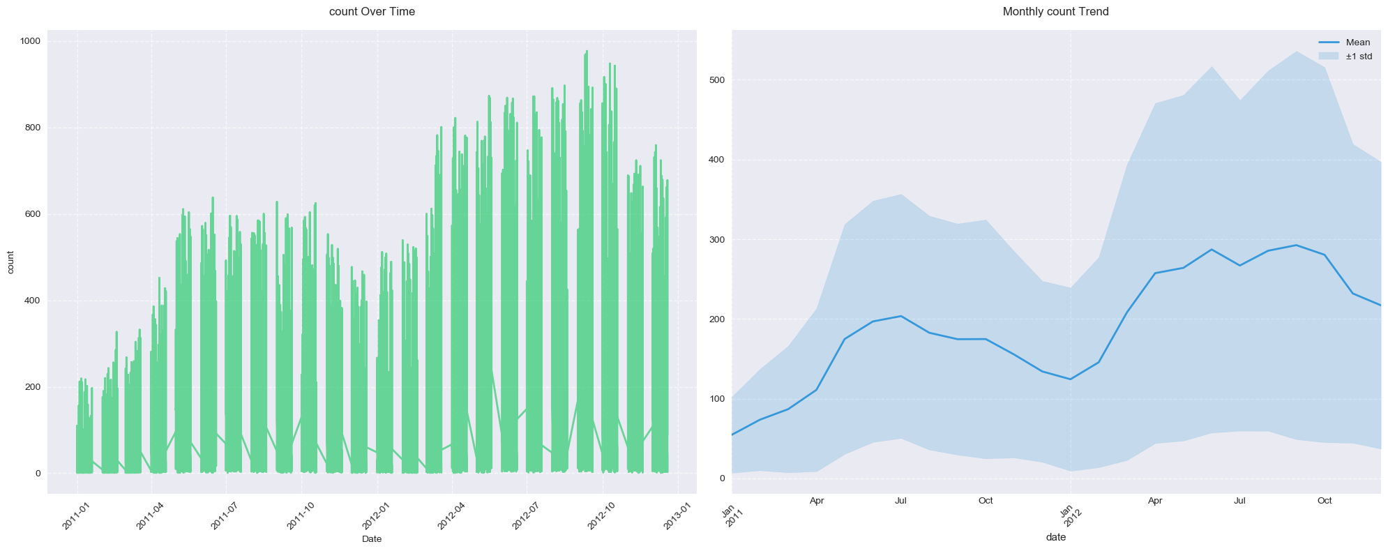
很明显,人们倾向于在夏季租用自行车,因为那个季节骑自行车的条件真的很好。因此,六月、七月和八月的自行车需求相对较高。
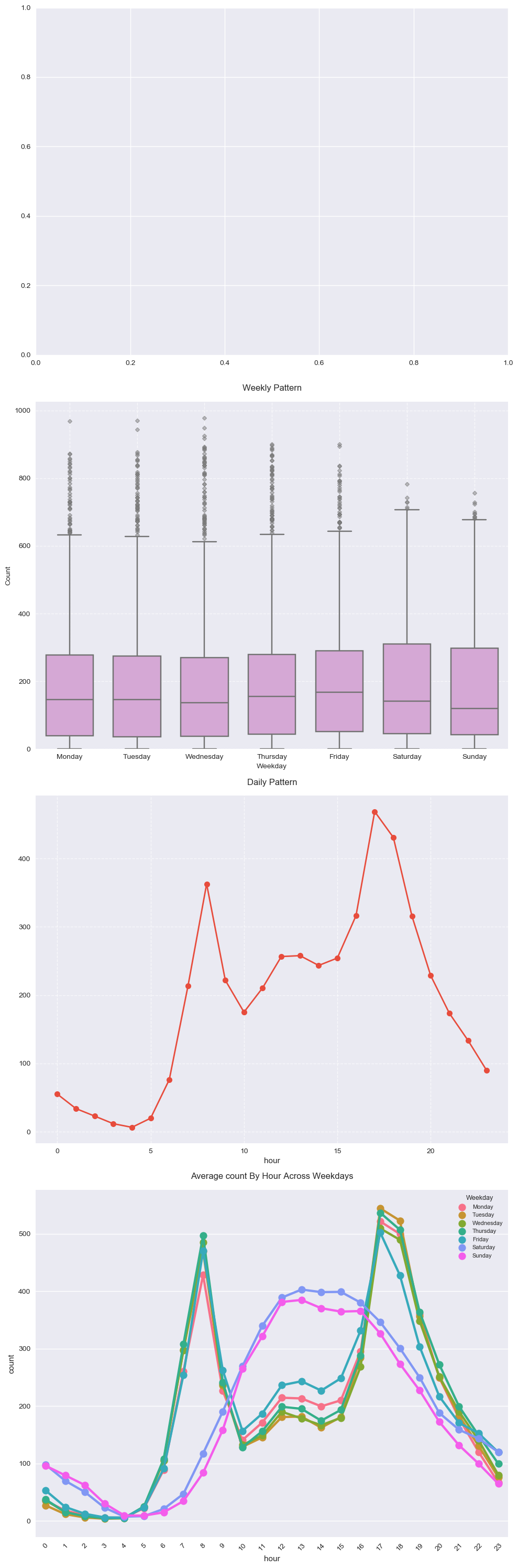
在工作日,更多人倾向于在上午7-8点和下午5-6点租用自行车。如前所述,这可以归因于常规的上学和上班通勤者。
在”周六”和”周日”没有观察到上述模式。更多人倾向于在上午10点到下午4点之间租用自行车。
1 2 3 4 5 6 7 8 9 10 11 12 13 14 15 16 17 18 19 20 21 22 23 24 25 26 27 28 29 30 31 32 33 34 35 36 37 38 39 40 41 42 43 44 45 46 47 48 49 50 51 52 53 54 55 56 57 58 59 60 61 62 63 64 65 66 67 68 69 70 71 72 73 74 75 76 77 78 79 80 81 82 83 def analyze_basic_time_series (data, target='count' , n_cols=2 , figsize=(20 , 8 ):""" 基础时间序列分析:展示目标变量随时间的整体趋势 参数: - data: DataFrame, 输入数据 - target: str, 目标变量名称 - n_cols: int, 图表列数 - figsize: tuple, 图形大小 """ 'seaborn' )if n_cols == 1 :'date' ], data[target], color='#2ecc71' , alpha=0.7 , linewidth=2 , label='Original' )'date' , inplace=True )'M' )'#3498db' , label='Monthly Mean' , linewidth=2 )'#3498db' ,0.2 ,'±1 std' f'{target} Over Time with Monthly Trend' , fontsize=12 , pad=15 )'Date' , fontsize=10 )10 )True , linestyle='--' , alpha=0.7 )'x' , rotation=45 )10 )else :1 , n_cols, figsize=figsize)0 ].plot(data['date' ], data[target], color='#2ecc71' , alpha=0.7 , linewidth=2 )0 ].set_title(f'{target} Over Time' , fontsize=12 , pad=15 )0 ].set_xlabel('Date' , fontsize=10 )0 ].set_ylabel(target, fontsize=10 )0 ].grid(True , linestyle='--' , alpha=0.7 )0 ].tick_params(axis='x' , rotation=45 )'date' , inplace=True )'M' )1 ], color='#3498db' , label='Mean' , linewidth=2 )1 ].fill_between('#3498db' ,0.2 ,'±1 std' 1 ].set_title(f'Monthly {target} Trend' , fontsize=12 , pad=15 )1 ].legend(fontsize=10 )1 ].grid(True , linestyle='--' , alpha=0.7 )1 ].tick_params(axis='x' , rotation=45 )'count' , n_cols=2 , figsize=(20 , 8 ))
1 2 3 4 5 6 7 8 9 10 11 12 13 14 15 16 17 18 19 20 21 22 23 24 25 26 27 28 29 30 31 32 33 34 35 36 37 38 39 40 41 42 43 44 45 46 47 48 49 50 51 52 53 54 55 56 57 58 59 60 def analyze_time_distributions (data, target='count' , n_cols=1 , figsize=(20 , 15 ):""" 时间分布分析:展示目标变量在不同时间维度上的分布 参数: - data: DataFrame, 输入数据 - target: str, 目标变量名称 - n_cols: int, 图表列数,默认为2 - figsize: tuple, 图形大小 """ 'seaborn' )3 1 ) // n_cols if n_rows == 1 :1 , -1 )elif n_cols == 1 :1 , 1 )'#3498db' , '#2ecc71' , '#e74c3c' , '#f1c40f' , '#9b59b6' ]for i in range (n_plots)]0 ]'year' , y=target, data=data, ax=axes[row, col], palette='husl' )f'{target} Distribution by Year' , fontsize=12 , pad=15 )10 )1 ]'month' , y=target, hue='quarter' , data=data, ax=axes[row, col], palette='husl' )f'{target} Distribution by Month and Quarter' , fontsize=12 , pad=15 )10 )2 ]'hour' , y=target, hue='is_weekend' , data=data, ax=axes[row, col], palette=['#3498db' , '#e74c3c' ])f'{target} Distribution by Hour and Weekend Status' , fontsize=12 , pad=15 )10 )for i in range (n_plots, n_rows * n_cols):'count' , n_cols=1 , figsize=(10 , 30 ))
1 2 3 4 5 6 7 8 9 10 11 12 13 14 15 16 17 18 19 20 21 22 23 24 25 26 27 28 29 30 31 32 33 34 35 36 37 38 39 40 41 42 43 44 45 46 47 48 49 50 51 52 53 54 55 56 57 58 59 60 61 62 63 64 65 66 67 68 69 70 71 72 73 74 75 76 77 78 79 80 81 82 83 84 85 86 87 88 89 90 91 92 93 94 95 96 97 98 99 100 101 102 103 104 105 106 107 108 109 110 111 112 113 114 115 116 117 118 119 120 121 122 123 124 125 126 127 128 129 130 131 132 133 134 135 136 137 138 139 140 141 142 143 144 145 146 147 148 149 150 151 def analyze_cyclical_patterns (data, target='count' , n_cols=2 , figsize=(20 , 15 ):'font.sans-serif' ] = ['SimHei' ] 'axes.unicode_minus' ] = False """ 时间周期模式分析:展示目标变量在不同周期上的变化模式 参数: - data: DataFrame, 输入数据 - target: str, 目标变量名称 - n_cols: int, 图表列数 - figsize: tuple, 图形大小 """ 'seaborn' )'weekday' : {0 :"Monday" , 1 :"Tuesday" , 2 :"Wednesday" , 3 :"Thursday" ,4 :"Friday" , 5 :"Saturday" , 6 :"Sunday" 4 1 ) // n_cols if n_rows == 1 :1 , -1 )elif n_cols == 1 :1 , 1 )'#3498db' , '#2ecc71' , '#e74c3c' , '#f1c40f' ]for i in range (n_plots)]1 ]'weekday' ,'plum' , 0.7 ,'marker' : 'D' ,'markerfacecolor' : 'gray' ,'markersize' : 4 ,'alpha' : 0.5 range (7 ))'Monday' , 'Tuesday' , 'Wednesday' , 'Thursday' , 'Friday' , 'Saturday' , 'Sunday' ],0 'Weekly Pattern' , fontsize=12 , pad=15 )'Weekday' , fontsize=10 )'Count' , fontsize=10 )True , linestyle='--' , alpha=0.7 )10 )0 )2 ]'hour' )[target].mean()'line' , 'o' ,2 ],2 ,8 'Daily Pattern' , fontsize=12 , pad=15 )True , linestyle='--' , alpha=0.7 )10 )3 ]"hour" ,"weekday" ], sort=True )[target].mean()'weekday' ] = hour_weekday_agg['weekday' ].map (feature_maps['weekday' ])"hour" , "weekday" , 'husl' f"Average {target} By Hour Across Weekdays" , fontsize=12 , pad=15 )'x' , rotation=45 , labelsize=10 )'Weekday' , 'upper right' , 1 , 1 ), 8 , 9 , 1 for i in range (n_plots, n_rows * n_cols):'count' , n_cols=1 , figsize=(10 , 30 ))
统计量分析- 单变量分析 数值型特征 描述性统计量
season
holiday
workingday
weather
temp
atemp
humidity
windspeed
casual
registered
count
year
month
day
hour
minute
weekday
quarter
is_weekend
count
10886.000000
10886.000000
10886.000000
10886.000000
10886.00000
10886.000000
10886.000000
10886.000000
10886.000000
10886.000000
10886.000000
10886.000000
10886.000000
10886.000000
10886.000000
10886.0
10886.000000
10886.000000
10886.000000
mean
2.506614
0.028569
0.680875
1.418427
20.23086
23.655084
61.886460
12.799395
36.021955
155.552177
191.574132
2011.501929
6.521495
9.992559
11.541613
0.0
3.013963
2.506614
0.290557
std
1.116174
0.166599
0.466159
0.633839
7.79159
8.474601
19.245033
8.164537
49.960477
151.039033
181.144454
0.500019
3.444373
5.476608
6.915838
0.0
2.004585
1.116174
0.454040
min
1.000000
0.000000
0.000000
1.000000
0.82000
0.760000
0.000000
0.000000
0.000000
0.000000
1.000000
2011.000000
1.000000
1.000000
0.000000
0.0
0.000000
1.000000
0.000000
25%
2.000000
0.000000
0.000000
1.000000
13.94000
16.665000
47.000000
7.001500
4.000000
36.000000
42.000000
2011.000000
4.000000
5.000000
6.000000
0.0
1.000000
2.000000
0.000000
50%
3.000000
0.000000
1.000000
1.000000
20.50000
24.240000
62.000000
12.998000
17.000000
118.000000
145.000000
2012.000000
7.000000
10.000000
12.000000
0.0
3.000000
3.000000
0.000000
75%
4.000000
0.000000
1.000000
2.000000
26.24000
31.060000
77.000000
16.997900
49.000000
222.000000
284.000000
2012.000000
10.000000
15.000000
18.000000
0.0
5.000000
4.000000
1.000000
max
4.000000
1.000000
1.000000
4.000000
41.00000
45.455000
100.000000
56.996900
367.000000
886.000000
977.000000
2012.000000
12.000000
19.000000
23.000000
0.0
6.000000
4.000000
1.000000
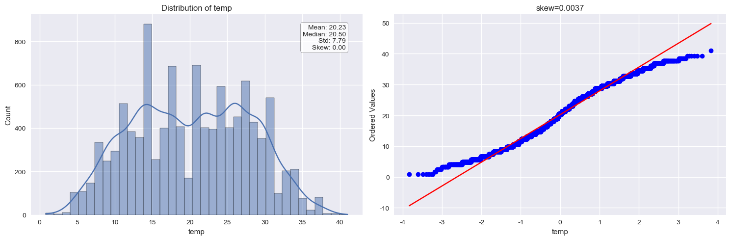
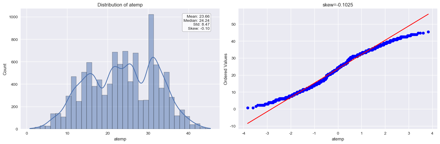
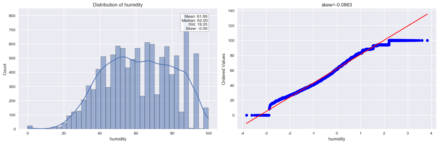
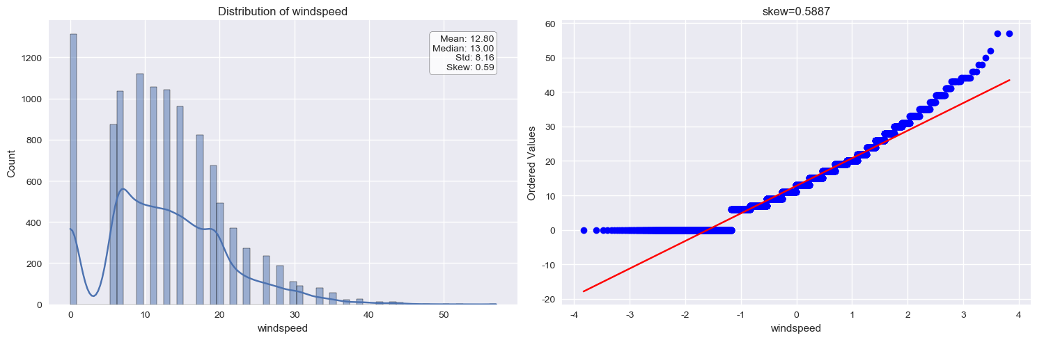
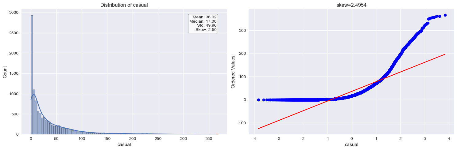
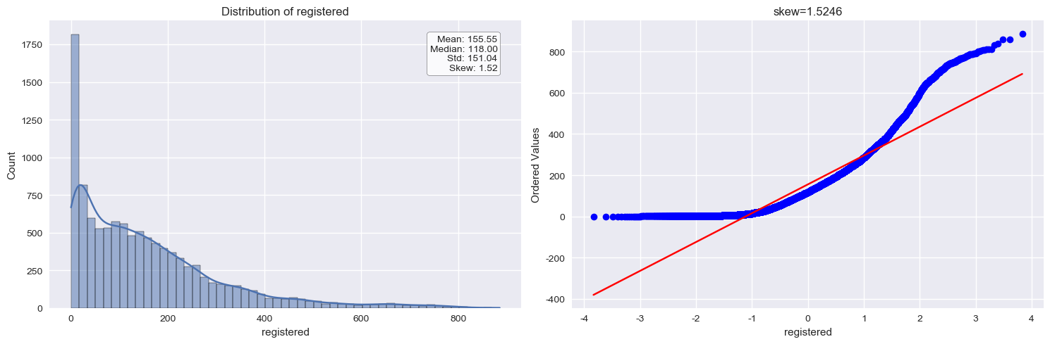
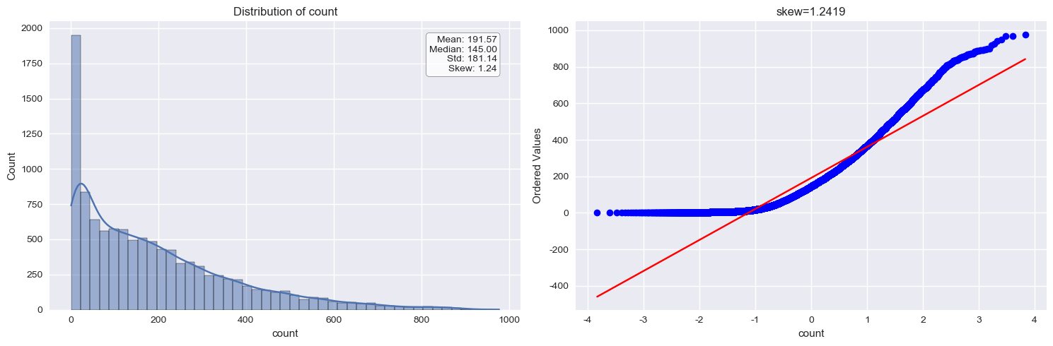
直方图和Q-Q图 从下图可以看出,”count”变量向右偏斜。由于大多数机器学习技术要求因变量呈正态分布,因此最好是正态分布。一个可能的解决方案是在删除异常数据点后对”count”变量进行对数转换。转换后的数据看起来好多了,但仍然不是完全理想的正态分布。
1 2 3 4 5 6 7 8 9 10 11 12 13 14 15 16 17 18 19 20 21 22 23 24 25 26 27 28 29 30 31 32 33 34 35 36 37 38 39 40 41 42 43 44 45 46 47 48 49 50 51 52 53 54 55 56 57 58 59 60 61 62 63 64 65 66 67 68 def plot_distributions (data, features=None , figsize=(15 , 5 ):""" 对数据集中的数值型特征进行分布可视化分析 参数: - data: DataFrame, 输入数据 - features: list, 需要分析的特征列表,默认为None(分析所有数值型特征) - figsize: tuple, 每个特征的图形大小,默认(15, 5) """ if features is None :'int64' , 'float64' ]).columnsimport warnings'ignore' , 'p-value may not be accurate for N > 5000' )for feature in features:if feature not in data.columns:print (f"警告: 特征 {feature} 不存在于数据集中" )continue if not np.issubdtype(data[feature].dtype, np.number):print (f"警告: 特征 {feature} 不是数值型变量" )continue 2 , nrows=1 , figsize=figsize)True , ax=ax1)f"Distribution of {feature} " )f"Mean: {data[feature].mean():.2 f} \n" f"Median: {data[feature].median():.2 f} \n" f"Std: {data[feature].std():.2 f} \n" f"Skew: {stats.skew(data[feature]):.2 f} " )0.95 , 0.95 , stats_info,'top' ,'right' ,dict (boxstyle='round' , facecolor='white' , alpha=0.8 ))'norm' , fit=True , plot=ax2)f"skew={stats.skew(data[feature]):.4 f} " )""" # 1. 分析所有数值型特征 plot_distributions(train_data) # 2. 分析指定特征 selected_features = ['temp', 'humidity', 'windspeed', 'count'] plot_distributions(train_data, features=selected_features) # 3. 自定义图形大小 plot_distributions(train_data, features=['count'], figsize=(12, 4)) """ 'temp' ,'atemp' ,'humidity' , 'windspeed' , 'casual' ,'registered' ,'count' ]
从这两张图可以得到以下重要信息:
从分布图(左图)可以看出:
数据分布严重右偏(right-skewed)
大部分租赁数量集中在较低值区域(0-200左右)
分布呈现长尾特征,有少量高值样本
不符合正态分布的形状
从Q-Q图(右图)可以看出:
数据点与红色参考线(表示理想的正态分布)有明显偏离
在两端的偏离特别明显,说明分布的尾部与正态分布差异较大
曲线呈现S形,进一步确认了数据的偏态性
后序处理:
对数据进行转换使其更接近正态分布
考虑使用能处理非正态分布的模型
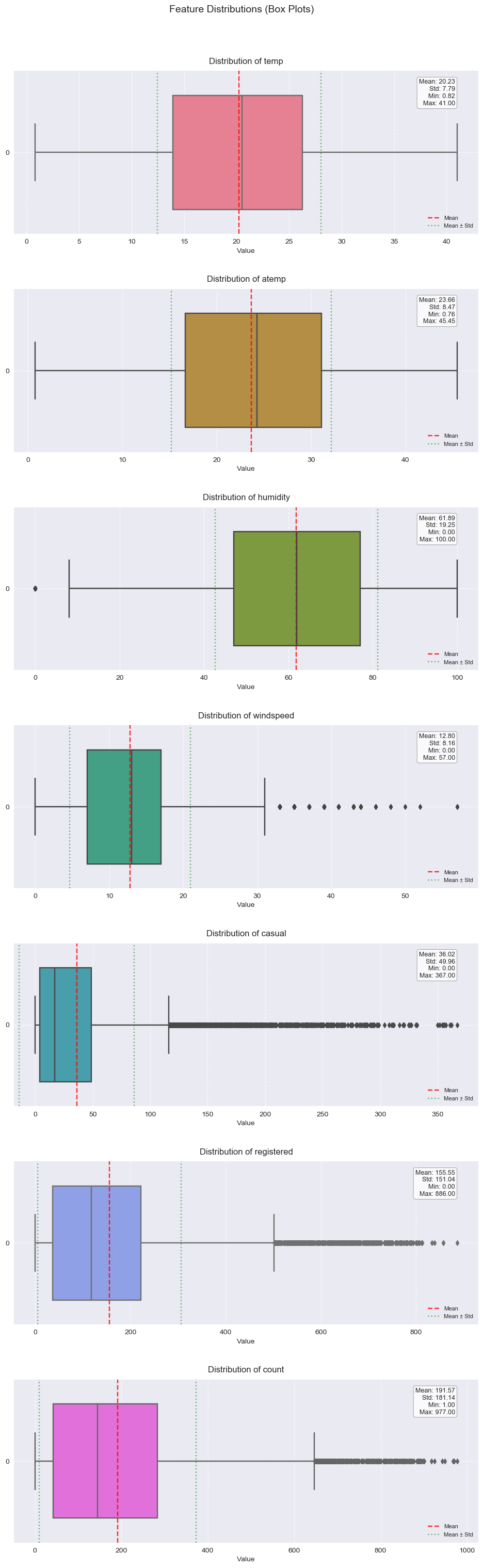
箱型图 1 2 3 4 5 6 7 8 9 10 11 12 13 14 15 16 17 18 19 20 21 22 23 24 25 26 27 28 29 30 31 32 33 34 35 36 37 38 39 40 41 42 43 44 45 46 47 48 49 50 51 52 53 54 55 56 57 58 59 60 61 62 63 64 65 66 67 68 69 70 71 72 73 74 75 76 77 78 79 80 81 82 83 84 85 86 87 88 89 90 91 92 93 94 95 96 97 98 def plot_boxplots (data, columns_to_plot, n_cols=2 ,figsize=(10 , 30 ):""" 绘制箱型图 参数: - data: DataFrame, 输入数据 - columns_to_plot: list, 需要绘制箱型图的列名列表 - n_cols: int, 子图列数 - figsize: tuple, 图形大小,默认根据特征数量自动调整 """ len (columns_to_plot)1 ) // n_cols + 1 if n_rows == 1 and n_cols == 1 :elif n_rows == 1 :1 , -1 )elif n_cols == 1 :1 , 1 )'seaborn' )"husl" , n_features)for i, (col, color) in enumerate (zip (columns_to_plot, colors)):"h" ,0.7 ,True , 'red' , linestyle='--' , alpha=0.8 , label='Mean' )'green' , linestyle=':' , alpha=0.5 , label='Mean ± Std' )'green' , linestyle=':' , alpha=0.5 )f'Distribution of {col} ' , 12 , 10 )'Value' , fontsize=10 )True , linestyle='--' , alpha=0.7 )10 )f'Mean: {stats["mean" ]:.2 f} \n' f'Std: {stats["std" ]:.2 f} \n' f'Min: {stats["min" ]:.2 f} \n' f'Max: {stats["max" ]:.2 f} ' )0.95 , 0.95 , stats_text,'top' ,'right' ,dict (boxstyle='round' , facecolor='white' , alpha=0.8 ),9 )'lower right' , fontsize=8 )for i in range (i + 1 , n_rows * n_cols):3.0 )'Feature Distributions (Box Plots)' , 14 , 1.02 )'temp' , 'atemp' , 'humidity' , 'windspeed' , 'casual' , 'registered' , 'count' ]1 )
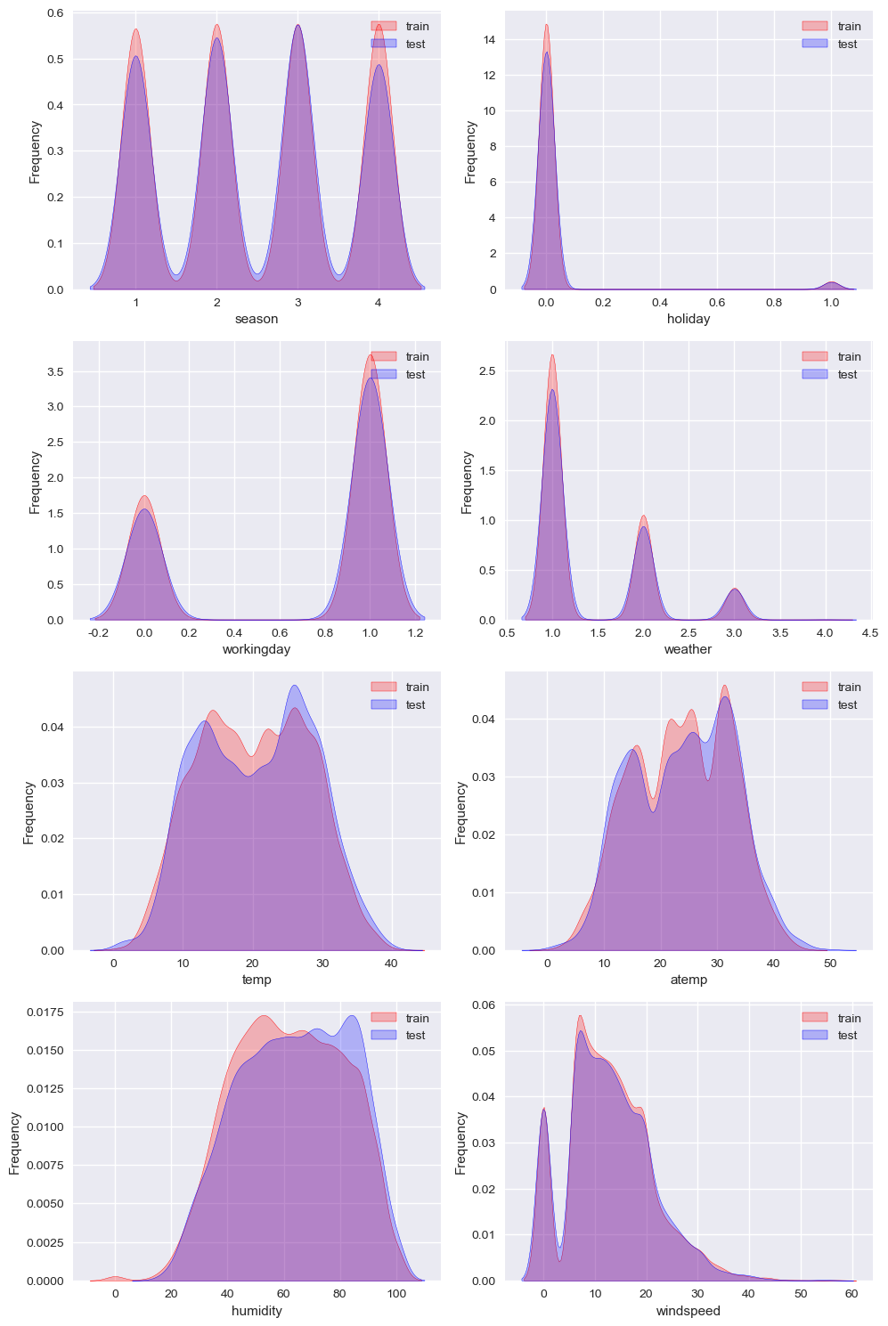
核密度估计图 KDE 1 2 3 4 5 6 7 8 9 10 11 12 13 14 15 16 17 18 19 20 21 22 23 24 25 26 27 28 29 30 31 32 33 34 35 36 37 38 39 40 41 42 43 44 45 46 47 48 49 50 51 52 53 54 55 56 57 58 59 60 61 62 63 64 65 66 67 68 69 70 71 72 73 74 75 76 77 78 79 80 81 82 83 84 85 86 87 88 89 90 91 92 93 94 95 96 97 98 99 100 101 102 103 104 105 106 107 108 109 110 def plot_kde_distributions (train_data, test_data, features_to_plot=None , figsize=None , n_cols=1 ):""" 绘制训练集和测试集的KDE分布对比图 参数: - train_data: DataFrame, 训练数据 - test_data: DataFrame, 测试数据 - features_to_plot: list, 需要绘制的特征列表。如果为None,则使用test_data的所有列 - figsize: tuple, 图形大小。如果为None,则自动计算 - n_cols: int, 图表列数,默认为1 """ if features_to_plot is None :'int64' , 'float64' ]).columnsfor feature in features_to_plot:if (feature not in train_data.columns or not in test_data.columns):print (f"警告: 特征 {feature} 不存在于训练集或测试集中" )continue if not pd.api.types.is_numeric_dtype(train_data[feature].astype(float )):print (f"警告: 特征 {feature} 不是数值型变量" )continue if not valid_features:print ("错误: 没有有效的数值型特征可以绘制" )return len (valid_features) + n_cols - 1 ) // n_colsif figsize is None :6 *n_cols, 4 *n_rows)if n_rows == 1 and n_cols == 1 :for i, col in enumerate (valid_features):float ),"Red" , True ,"train" ,float ),"Blue" , True ,"test" ,"Frequency" )for j in range (i+1 , len (axes)):False )""" # 1. 默认单列显示 plot_kde_distributions(train_data, test_data) # 2. 双列显示 plot_kde_distributions( train_data, test_data, n_cols=2, figsize=(15, 20) ) # 3. 三列显示特定特征 features_to_plot = ['temp', 'humidity', 'windspeed', 'casual', 'registered', 'count'] plot_kde_distributions( train_data, test_data, features_to_plot=features_to_plot, n_cols=3, figsize=(18, 8) ) """ "season" ,"holiday" ,"workingday" ,"weather" ,"temp" ,"atemp" ,"humidity" ,"windspeed" ]2 ,10 , 15 )
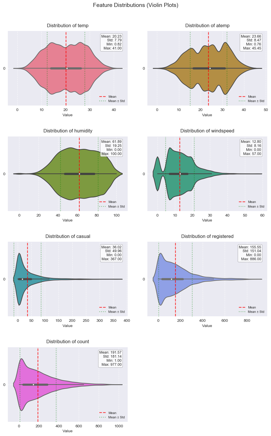
小提琴图 1 2 3 4 5 6 7 8 9 10 11 12 13 14 15 16 17 18 19 20 21 22 23 24 25 26 27 28 29 30 31 32 33 34 35 36 37 38 39 40 41 42 43 44 45 46 47 48 49 50 51 52 53 54 55 56 57 58 59 60 61 62 63 64 65 66 67 68 69 70 71 72 73 74 75 76 77 78 79 80 81 82 83 84 85 86 87 88 89 90 91 92 93 94 95 96 97 def plot_violinplots (data, columns_to_plot, n_cols=2 ,figsize=(10 , 30 ):""" 绘制小提琴图 参数: - data: DataFrame, 输入数据 - columns_to_plot: list, 需要绘制小提琴图的列名列表 - n_cols: int, 子图列数 - figsize: tuple, 图形大小,默认根据特征数量自动调整 """ len (columns_to_plot)1 ) // n_cols + 1 if n_rows == 1 and n_cols == 1 :elif n_rows == 1 :1 , -1 )elif n_cols == 1 :1 , 1 )'seaborn' )"husl" , n_features)for i, (col, color) in enumerate (zip (columns_to_plot, colors)):"h" ,0.7 ,'red' , linestyle='--' , alpha=0.8 , label='Mean' )'green' , linestyle=':' , alpha=0.5 , label='Mean ± Std' )'green' , linestyle=':' , alpha=0.5 )f'Distribution of {col} ' , 12 , 10 )'Value' , fontsize=10 )True , linestyle='--' , alpha=0.7 )10 )f'Mean: {stats["mean" ]:.2 f} \n' f'Std: {stats["std" ]:.2 f} \n' f'Min: {stats["min" ]:.2 f} \n' f'Max: {stats["max" ]:.2 f} ' )0.95 , 0.95 , stats_text,'top' ,'right' ,dict (boxstyle='round' , facecolor='white' , alpha=0.8 ),9 )'lower right' , fontsize=8 )for i in range (i + 1 , n_rows * n_cols):3.0 )'Feature Distributions (Violin Plots)' , 14 , 1.02 )'temp' , 'atemp' , 'humidity' , 'windspeed' , 'casual' , 'registered' , 'count' ]2 ,figsize=(10 ,15 ))
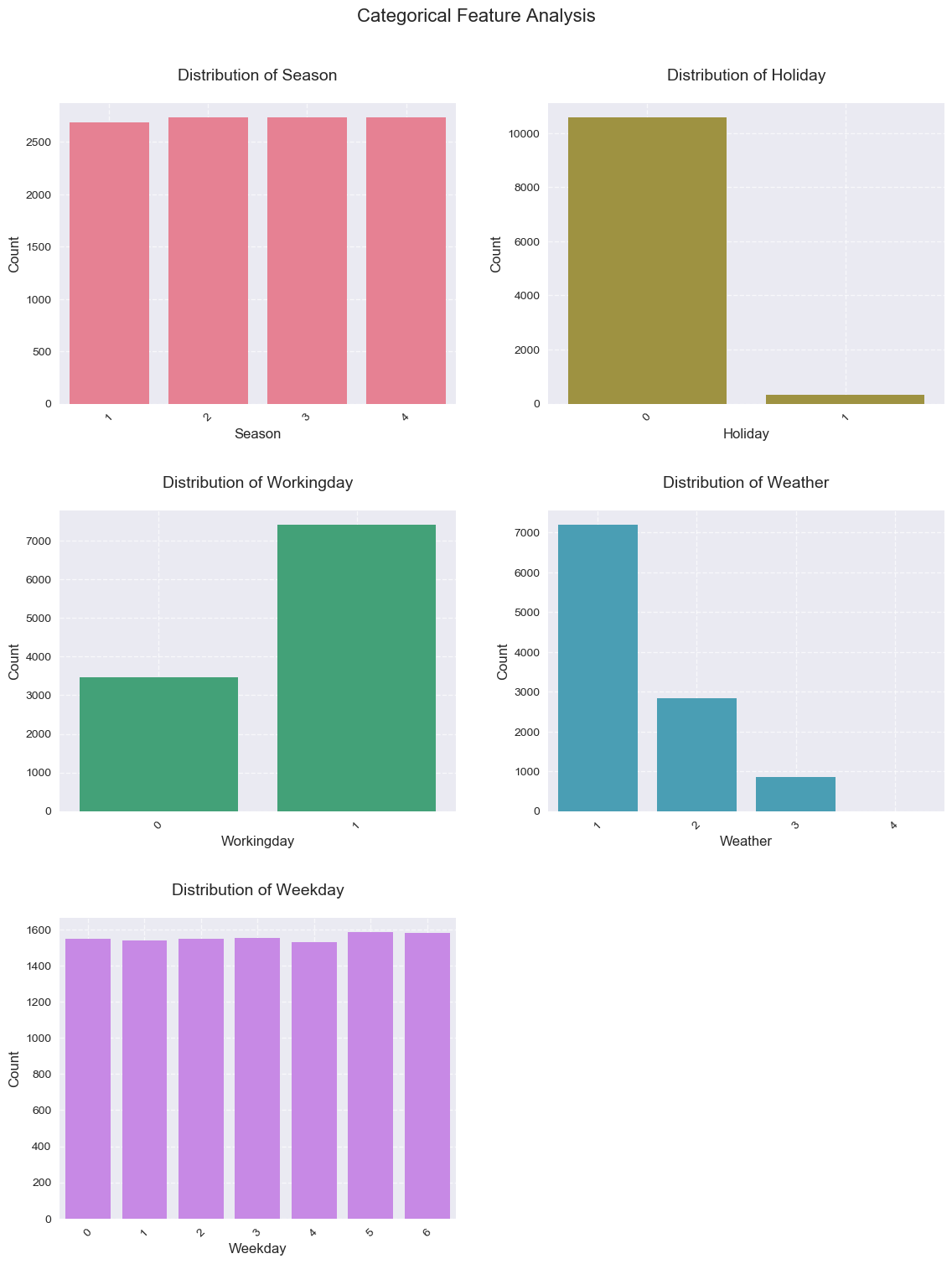
类别型特征 描述性统计量及条形图 1 2 3 4 5 6 7 8 9 10 11 12 13 14 15 16 17 18 19 20 21 22 23 24 25 26 27 28 29 30 31 32 33 34 35 36 37 38 39 40 41 42 43 44 45 46 47 48 49 50 51 52 53 54 55 56 57 58 59 60 61 62 63 64 65 66 67 68 69 70 71 72 73 74 75 76 77 78 79 80 81 82 83 84 85 86 87 88 89 90 91 92 93 94 95 96 97 98 99 100 101 102 103 104 105 106 107 108 109 110 111 112 113 114 115 116 117 118 119 120 121 122 123 124 125 126 127 128 129 130 131 132 133 134 135 136 137 138 139 140 141 142 143 def analyze_categorical_features (data, categorical_features=None , target=None , n_cols=2 , figsize=None ):""" 分析类别型特征的描述性统计量和可视化 参数: - data: DataFrame, 输入数据 - categorical_features: list or None, 需要分析的类别型特征列表,默认为None(自动选择) - target: str or None, 目标变量名,默认为None - n_cols: int, 子图列数,默认为2 - figsize: tuple or None, 图形大小,默认为None(自动计算大小) """ if categorical_features is None :'object' , 'category' , 'int64' ]).columns.tolist()if target in categorical_features:print (f"自动检测到的分类特征: {categorical_features} " )for feature in categorical_features:if feature not in data.columns:print (f"警告: 特征 {feature} 不存在" )continue if n_unique > 50 :print (f"警告: {feature} 的唯一值过多({n_unique} )" )continue if not valid_features:print ("错误: 没有有效的分类特征" )return len (valid_features)1 ) // n_colsif figsize is None :6 * n_cols5 * n_rowsif n_rows == 1 and n_cols == 1 :elif n_rows == 1 :1 , -1 )elif n_cols == 1 :1 , 1 )'seaborn' )"husl" , n_features)for idx, (feature, color) in enumerate (zip (valid_features, colors)):if n_rows > 1 or n_cols > 1 else axes[col]True ) * 100 'Count' : value_counts,'Percentage' : percentagesprint (f"\n=== {feature.capitalize()} 的描述性统计 ===" )print (stats_df)'Count' ,f'Distribution of {feature.capitalize()} ' , fontsize=14 , pad=20 )12 )'Count' , fontsize=12 )'both' , labelsize=10 )'x' , rotation=45 )True , linestyle='--' , alpha=0.7 )if n_features % n_cols != 0 and (n_rows > 1 or n_cols > 1 ):for j in range (n_features, n_rows * n_cols):3.0 )'Categorical Feature Analysis' , 16 , 1.02 """ # 基本使用 analyze_categorical_features(train_data) # 指定特征 analyze_categorical_features( data=train_data, categorical_features=['season', 'holiday', 'workingday', 'weather'] ) # 自定义大小 analyze_categorical_features( data=train_data, categorical_features=['hour', 'weekday', 'month'], figsize=(15, 20) ) """ 'season' ,'holiday' , 'workingday' ,'weather' ,'weekday' ]2
=== Season 的描述性统计 ===
Count Percentage
4 2734 25.114826
2 2733 25.105640
3 2733 25.105640
1 2686 24.673893
=== Holiday 的描述性统计 ===
Count Percentage
0 10575 97.14312
1 311 2.85688
=== Workingday 的描述性统计 ===
Count Percentage
1 7412 68.087452
0 3474 31.912548
=== Weather 的描述性统计 ===
Count Percentage
1 7192 66.066507
2 2834 26.033437
3 859 7.890869
4 1 0.009186
=== Weekday 的描述性统计 ===
Count Percentage
5 1584 14.550799
6 1579 14.504869
3 1553 14.266030
0 1551 14.247658
2 1551 14.247658
1 1539 14.137424
4 1529 14.045563
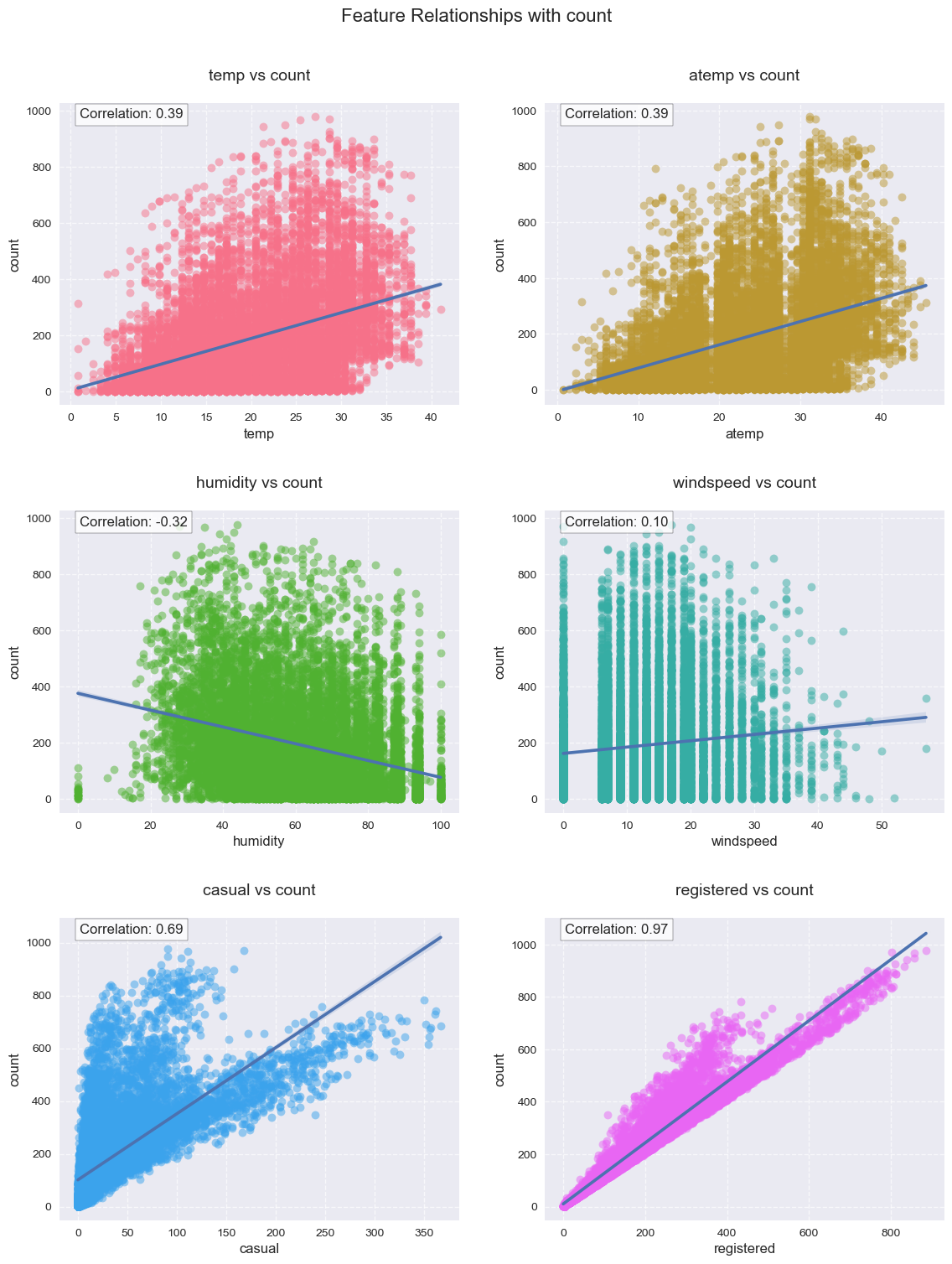
统计量分析- 双变量/多变量分析 1. 数值型特征 vs. 数值型特征 散点图 1 2 3 4 5 6 7 8 9 10 11 12 13 14 15 16 17 18 19 20 21 22 23 24 25 26 27 28 29 30 31 32 33 34 35 36 37 38 39 40 41 42 43 44 45 46 47 48 49 50 51 52 53 54 55 56 57 58 59 60 61 62 63 64 65 66 67 68 69 70 71 72 73 74 75 76 77 78 79 80 81 82 83 84 85 86 87 88 89 90 91 92 93 94 95 96 97 98 99 100 101 102 103 104 105 106 107 108 109 110 111 112 113 114 115 116 117 118 119 120 121 122 123 124 125 126 127 128 129 130 131 132 133 134 135 136 137 def plot_feature_target_relationships (data, features_to_plot=None , target='count' , figsize=None , n_cols=1 ):""" 绘制特征与目标变量的关系图,支持自定义布局 参数: - data: DataFrame, 输入数据 - features_to_plot: list or None, 需要绘制的特征列表,默认为None(自动选择数值特征) - target: str, 目标变量名,默认为'count' - figsize: tuple or None, 图形大小,默认为None(自动计算大小) - n_cols: int, 子图列数,默认为1 """ if features_to_plot is None :'int64' , 'float64' ]).columns.tolist()if target in features_to_plot:len (features_to_plot)1 ) // n_cols + 1 if figsize is None :6 * n_cols 5 * n_rows if n_rows == 1 and n_cols == 1 :elif n_rows == 1 :1 , -1 )elif n_cols == 1 :1 , 1 )'seaborn' )"husl" , n_features)for idx, (feature, color) in enumerate (zip (features_to_plot, colors)):'alpha' : 0.5 ,'s' : 50 ,'color' : colorf'{feature} vs {target} ' , fontsize=14 , pad=20 )12 )12 )'both' , labelsize=10 )True , linestyle='--' , alpha=0.7 )0 , 1 ]0.05 , 0.95 , f'Correlation: {corr:.2 f} ' ,12 ,dict (facecolor='white' , alpha=0.8 )for idx in range (n_features, n_rows * n_cols):3.0 )f'Feature Relationships with {target} ' , 16 , 1.02 """ # 1. 默认单列布局 plot_feature_target_relationships(train_data) # 2. 双列布局 plot_feature_target_relationships(train_data, n_cols=2) # 3. 三列布局并自定义大小 plot_feature_target_relationships( train_data, n_cols=3, figsize=(20, 15) ) # 4. 完整自定义 features = ['temp', 'atemp', 'humidity', 'windspeed'] plot_feature_target_relationships( data=train_data, features_to_plot=features, target='registered', n_cols=2, figsize=(15, 10) ) """ 'temp' , 'atemp' , 'humidity' , 'windspeed' , 'casual' , 'registered' ]'count' ,2 ,
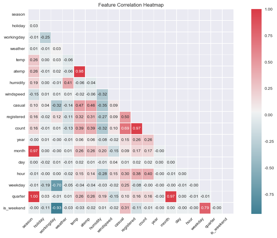
热力图 1 2 3 4 5 6 7 8 9 10 11 12 13 14 15 16 17 18 19 20 21 22 23 24 25 26 27 28 29 30 31 32 33 34 35 36 37 38 39 40 41 42 43 44 45 46 47 48 49 50 51 52 53 54 55 56 57 58 59 60 61 62 63 64 65 66 67 68 69 70 71 72 73 74 75 76 77 78 79 80 81 82 83 84 85 86 87 88 89 90 91 92 93 94 95 96 97 98 99 100 101 102 103 104 105 106 107 108 109 110 111 112 113 114 115 116 117 118 119 120 121 122 123 124 125 126 127 128 129 130 131 132 133 134 135 136 137 138 139 140 141 142 143 144 145 146 147 148 149 150 151 def analyze_feature_correlations ( data, target='target' , k=10 , threshold=0.5 , figsize=(12 , 8 exclude_features=None """ 分析特征与目标变量的相关性 参数: - data: DataFrame, 输入数据 - target: str, 目标变量名 - k: int, 选择最相关的特征数量 - threshold: float, 相关系数阈值 - figsize: tuple, 图形大小 - exclude_features: list, 要排除的特征列表,默认为None 返回: - dict: 包含分析结果的字典 """ if exclude_features is None :if target in exclude_features:print (f"警告:目标变量 {target} 已从排除列表中移除" )for col in data.columns if col not in exclude_features]'extremely_strong' : 0.7 , 'strong' : 0.5 , 'moderate' : 0.3 , 'weak' : 0.1 bool )True 220 , 10 , as_cmap=True )True ,True ,'.2f' ,True ,.5 ,'white' 'Feature Correlation Heatmap' )45 , ha='right' ) 0 )False )'extremely_strong' : [],'strong' : [],'moderate' : [],'weak' : [],'very_weak' : []for feature, corr in target_correlations.items():if feature == target:continue abs (corr)if abs_corr >= correlation_thresholds['extremely_strong' ]:'extremely_strong' ].append((feature, corr))elif abs_corr >= correlation_thresholds['strong' ]:'strong' ].append((feature, corr))elif abs_corr >= correlation_thresholds['moderate' ]:'moderate' ].append((feature, corr))elif abs_corr >= correlation_thresholds['weak' ]:'weak' ].append((feature, corr))else :'very_weak' ].append((feature, corr))abs (corr_matrix[target]) > threshold]abs ().sort_values(ascending=False ).indexlist (set (high_corr_series.index).intersection(set (top_k_features)))print ("\n=== 特征相关性分析结果 ===" )if exclude_features:print (f"\n已排除的特征 ({len (exclude_features)} 个):" )print (exclude_features)print (f"\n1. 相关系数大于 {threshold} 的特征 ({len (high_corr_features)} 个):" )print (high_corr_series.index.tolist())print (f"\n2. 相关性最强的前 {k} 个特征:" )print (top_k_features.tolist())print ("\n3. 同时满足以上两个条件的特征:" )print (common_features)print ("\n4. 按相关性强度划分的特征:" )for category, features in correlation_categories.items():if features:print (f"\n{category.replace('_' , ' ' ).title()} Correlation (|r| >= {correlation_thresholds.get(category, 0 )} ):" )for feature, corr in features:print (f"{feature} : {corr:.4 f} " )return {'high_corr_features' : high_corr_series.index,'top_k_features' : top_k_features,'target_correlations' : target_correlations,'common_features' : common_features,'correlation_categories' : correlation_categories,'excluded_features' : exclude_features 'count' ,5 ,0.3 ,'minute' ,'is_month_end' ]
已排除的特征 (2个):
['minute', 'is_month_end']
1. 相关系数大于 0.3 的特征 (7个):
['count', 'registered', 'casual', 'hour', 'temp', 'atemp', 'humidity']
2. 相关性最强的前 5 个特征:
['count', 'registered', 'casual', 'hour', 'temp']
3. 同时满足以上两个条件的特征:
['temp', 'hour', 'count', 'registered', 'casual']
4. 按相关性强度划分的特征:
Extremely Strong Correlation (|r| >= 0.7):
registered: 0.9709
Strong Correlation (|r| >= 0.5):
casual: 0.6904
Moderate Correlation (|r| >= 0.3):
hour: 0.4006
temp: 0.3945
atemp: 0.3898
humidity: -0.3174
Weak Correlation (|r| >= 0.1):
year: 0.2604
month: 0.1669
quarter: 0.1634
season: 0.1634
windspeed: 0.1014
weather: -0.1287
Very Weak Correlation (|r| >= 0):
day: 0.0198
workingday: 0.0116
weekday: -0.0023
holiday: -0.0054
is_weekend: -0.0099
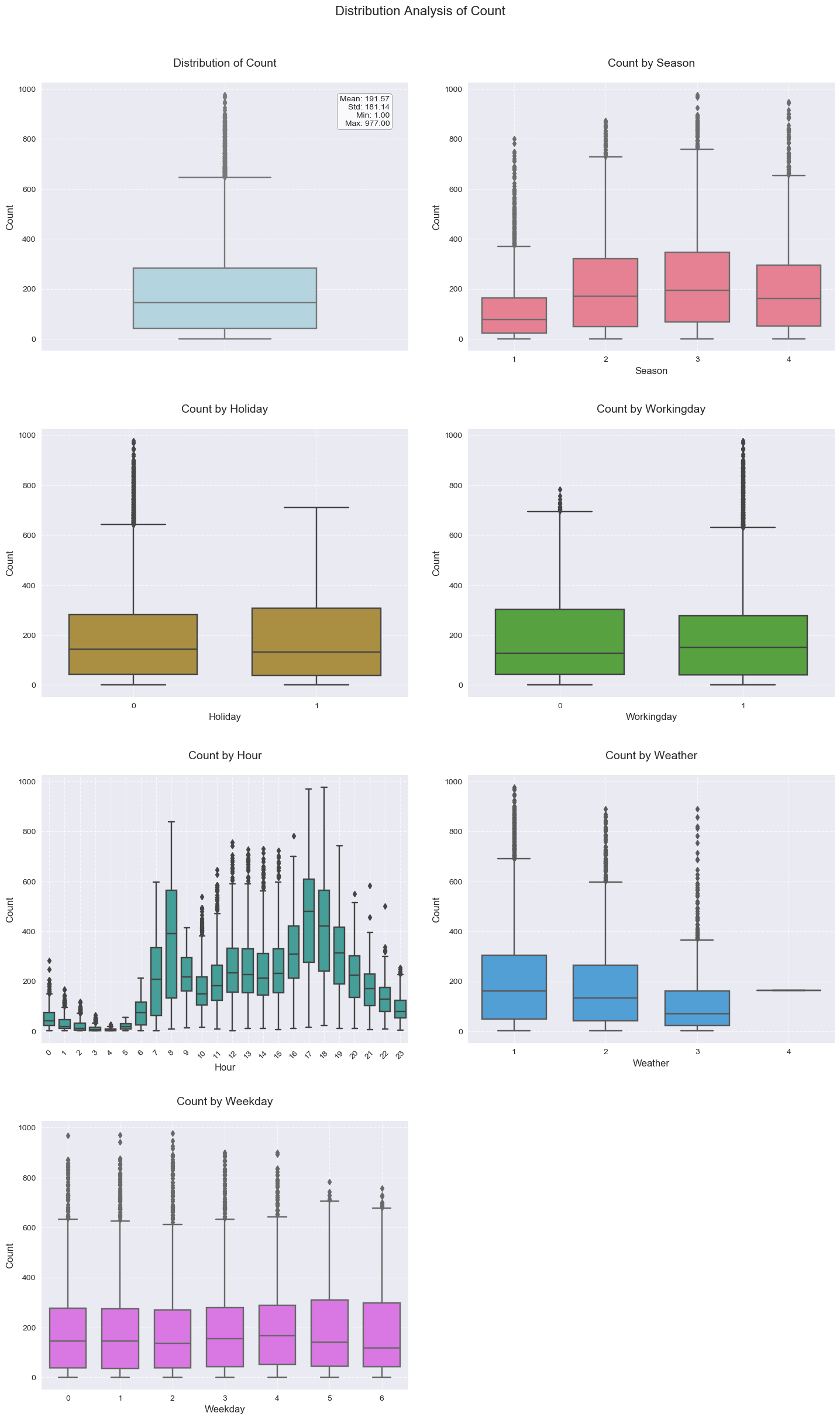
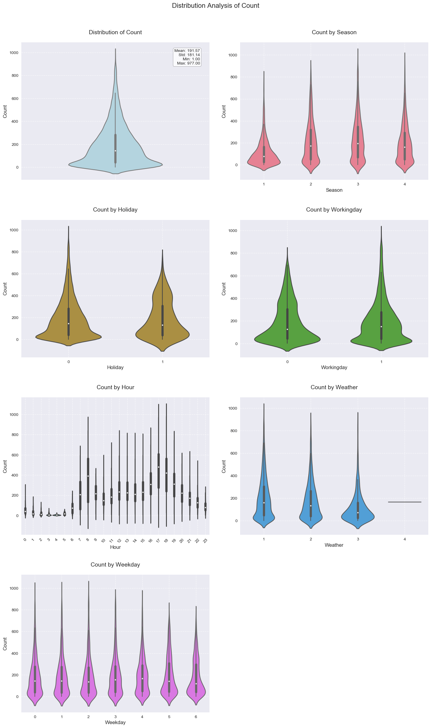
2. 类别型特征 vs. 数值型特征 箱线图 (Box Plot) 和小提琴图 初看之下,”count”变量包含许多异常数据点,这使得分布向右偏斜(因为有更多的数据点超出了外四分位限)。但除此之外,从下面的简单箱线图中还可以得出以下结论:
春季的租赁数量相对较低。箱线图中位数值的下降证实了这一点。
“每日小时数”的箱线图非常有趣。在上午7-8点和下午5-6点,中位数值相对较高。这可以归因于该时段的常规上学和上班用户。
大多数异常点主要来自”工作日”而不是”非工作日”。从图4中可以清楚地看到这一点。
1
2
3
4
5
6
7
8
9
10
11
12
13
14
15
16
17
18
19
20
21
22
23
24
25
26
27
28
29
30
31
32
33
34
35
36
37
38
39
40
41
42
43
44
45
46
47
48
49
50
51
52
53
54
55
56
57
58
59
60
61
62
63
64
65
66
67
68
69
70
71
72
73
74
75
76
77
78
79
80
81
82
83
84
85
86
87
88
89
90
91
92
93
94
95
96
97
98
99
100
101
102
103
104
105
106
107
108
109
110
111
112
113
114
115
116
117
118
119
120
121
122
123
124
125
126
127
128
129
130
131
132
133
134
135
136
137
138
139
140
141
142
143
144
145
146
147
148
149
150
151
def plot_boxplots_with_target (data, target, categorical_features=None , figsize=None ):""" 绘制优化版本的目标变量箱型图分析 参数: - data: DataFrame, 输入数据 - target: str, 目标变量名称 - categorical_features: list or None, 分类特征列表 - figsize: tuple or None, 图形大小,默认根据特征数量自动计算 """ if categorical_features is None :'object' , 'category' , 'int64' ]).columnsfor col in categorical_features if col != target]print (f"自动检测到的分类特征: {categorical_features} " )for feature in categorical_features:if feature not in data.columns:print (f"警告: 特征 {feature} 不存在" )continue if n_unique > 50 :print (f"警告: {feature} 的唯一值过多({n_unique} )" )continue if not valid_features:print ("错误: 没有有效的分类特征" )return len (valid_features) + 1 2 1 ) // n_colsif figsize is None :15 , 6 * n_rows) 'seaborn' )"v" ,0 ][0 ],'lightblue' ,0.5 0 ][0 ].set_title(f'Distribution of {target.capitalize()} ' , 14 , pad=20 )0 ][0 ].set_ylabel(target.capitalize(), fontsize=12 )0 ][0 ].tick_params(labelsize=10 )0 ][0 ].grid(True , linestyle='--' , alpha=0.7 )f'Mean: {stats["mean" ]:.2 f} \n' f'Std: {stats["std" ]:.2 f} \n' f'Min: {stats["min" ]:.2 f} \n' f'Max: {stats["max" ]:.2 f} ' )0 ][0 ].text(0.95 , 0.95 , stats_text,0 ][0 ].transAxes,'top' ,'right' ,dict (boxstyle='round' , facecolor='white' , alpha=0.8 ),10 "husl" , len (valid_features))for i, (feature, color) in enumerate (zip (valid_features, colors)):1 ) // 2 1 ) % 2 "v" ,0.7 f'{target.capitalize()} by {feature.capitalize()} ' , 14 , pad=20 )12 )12 )'both' , labelsize=10 )if len (data[feature].unique()) > 10 :'x' , rotation=45 )True , linestyle='--' , alpha=0.7 )if len (valid_features) % 2 == 0 :1 ][1 ])3.0 )f'Distribution Analysis of {target.capitalize()} ' , 16 , 1.02 """ # 基本使用 plot_boxplots_with_target(train_data, target='count') # 指定特征 plot_boxplots_with_target( data=train_data, target='count', categorical_features=['season', 'holiday', 'workingday', 'weather'] ) # 自定义大小 plot_boxplots_with_target( data=train_data, target='count', categorical_features=['hour', 'weekday', 'month'], figsize=(15, 20) ) """ 'count' ,'season' ,'holiday' , 'workingday' ,'hour' ,'weather' ,'weekday' ]
1 2 3 4 5 6 7 8 9 10 11 12 13 14 15 16 17 18 19 20 21 22 23 24 25 26 27 28 29 30 31 32 33 34 35 36 37 38 39 40 41 42 43 44 45 46 47 48 49 50 51 52 53 54 55 56 57 58 59 60 61 62 63 64 65 66 67 68 69 70 71 72 73 74 75 76 77 78 79 80 81 82 83 84 85 86 87 88 89 90 91 92 93 94 95 96 97 98 99 100 101 102 103 104 105 106 107 108 109 110 111 112 113 114 115 116 117 118 119 120 121 122 123 124 125 126 127 128 129 130 131 132 133 134 135 136 137 138 139 140 141 142 143 144 145 146 147 148 149 150 151 152 153 154 155 156 157 158 159 160 161 162 163 164 165 166 def plot_boxplots_with_target (data, target, categorical_features=None , n_cols=2 , figsize=None , violin_width=0.7 ):""" 绘制目标变量小提琴图分析 参数: - data: DataFrame, 输入数据 - target: str, 目标变量名称 - categorical_features: list or None, 分类特征列表 - n_cols: int, 子图列数,默认为2 - figsize: tuple or None, 图形大小,默认根据特征数量自动计算 - violin_width: float, 小提琴图的宽度,默认为0.7 """ if categorical_features is None :'object' , 'category' , 'int64' ]).columnsfor col in categorical_features if col != target]print (f"自动检测到的分类特征: {categorical_features} " )for feature in categorical_features:if feature not in data.columns:print (f"警告: 特征 {feature} 不存在" )continue if n_unique > 50 :print (f"警告: {feature} 的唯一值过多({n_unique} )" )continue if not valid_features:print ("错误: 没有有效的分类特征" )return len (valid_features) + 1 1 ) // n_cols if figsize is None :15 , 6 * n_rows) 'seaborn' )if n_rows == 1 and n_cols == 1 :elif n_rows == 1 :1 , -1 )elif n_cols == 1 :1 , 1 )"v" ,0 ][0 ] if n_rows > 1 or n_cols > 1 else axes[0 ], 'lightblue' ,0.5 0 ][0 ] if n_rows > 1 or n_cols > 1 else axes[0 ]f'Distribution of {target.capitalize()} ' , 14 , pad=20 )12 )10 )True , linestyle='--' , alpha=0.7 )f'Mean: {stats["mean" ]:.2 f} \n' f'Std: {stats["std" ]:.2 f} \n' f'Min: {stats["min" ]:.2 f} \n' f'Max: {stats["max" ]:.2 f} ' )0.95 , 0.95 , stats_text,'top' ,'right' ,dict (boxstyle='round' , facecolor='white' , alpha=0.8 ),10 "husl" , len (valid_features))for i, (feature, color) in enumerate (zip (valid_features, colors)):1 ) // n_cols1 ) % n_colsif n_rows > 1 or n_cols > 1 else axes[col]"v" ,if feature != 'hour' else violin_width * 1.5 f'{target.capitalize()} by {feature.capitalize()} ' , 14 , pad=20 )12 )12 )'both' , labelsize=10 )if len (data[feature].unique()) > 10 :'x' , rotation=45 )True , linestyle='--' , alpha=0.7 )if n_plots % n_cols != 0 and (n_rows > 1 or n_cols > 1 ):for j in range (n_plots, n_rows * n_cols):3.0 )f'Distribution Analysis of {target.capitalize()} ' , 16 , 1.02 """ # 基本使用 plot_boxplots_with_target(train_data, target='count') # 指定特征 plot_boxplots_with_target( data=train_data, target='count', categorical_features=['season', 'holiday', 'workingday', 'weather'] ) # 自定义大小 plot_boxplots_with_target( data=train_data, target='count', categorical_features=['hour', 'weekday', 'month'], figsize=(15, 20) ) """ 'count' ,'season' ,'holiday' , 'workingday' ,'hour' ,'weather' ,'weekday' ],2 ,
3. 类别型特征 vs. 类别型特征 交叉表 1 2 3 4 5 6 7 8 9 10 11 12 13 14 15 16 17 18 19 20 21 22 23 24 25 26 27 28 29 30 31 32 33 34 35 36 37 38 39 40 41 42 43 44 45 46 47 48 49 50 51 52 53 54 55 56 57 58 59 60 61 62 63 64 65 66 67 68 69 70 71 72 73 74 75 76 77 78 79 80 81 82 83 84 85 86 87 88 89 90 91 92 93 94 95 96 97 def plot_categorical_relationship (data, cat_features, n_cols=2 , figsize=None ):""" 绘制类别型特征之间的交叉表 参数: - data: DataFrame, 输入数据 - cat_features: list, 需要分析的两个类别型特征列表 - n_cols: int, 子图列数,默认为2 - figsize: tuple or None, 图形大小,默认为None(自动计算大小) """ if len (cat_features) != 2 :print ("错误: 请提供两个类别型特征进行分析" )return for feature in cat_features:if feature not in data.columns:print (f"警告: 特征 {feature} 不存在" )return if n_unique > 50 :print (f"警告: {feature} 的唯一值过多({n_unique} )" )return 1 1 ) // n_colsif figsize is None :10 * n_cols6 * n_rowsif n_rows == 1 and n_cols == 1 :elif n_rows == 1 :1 , -1 )0 ][0 ]elif n_cols == 1 :1 , 1 )0 ][0 ]else :0 ][0 ]'seaborn' )0 ]], data[cat_features[1 ]])True , fmt='d' , cmap='Blues' , ax=ax_cross)f'Crosstab of {cat_features[0 ].capitalize()} vs {cat_features[1 ].capitalize()} ' , fontsize=14 , pad=20 )1 ].capitalize(), fontsize=12 )0 ].capitalize(), fontsize=12 )'both' , labelsize=10 )if n_plots % n_cols != 0 and (n_rows > 1 or n_cols > 1 ):for j in range (n_plots, n_rows * n_cols):3.0 )f'Relationship Analysis of {cat_features[0 ].capitalize()} and {cat_features[1 ].capitalize()} ' , 16 , 1.02 """ # 基本使用 plot_categorical_relationship(train_data, cat_features=['season', 'weather']) # 自定义大小 plot_categorical_relationship( data=train_data, cat_features=['weekday', 'hour'], figsize=(15, 10) ) """
"\n# 基本使用\nplot_categorical_relationship(train_data, cat_features=['season', 'weather'])\n\n# 自定义大小\nplot_categorical_relationship(\n data=train_data,\n cat_features=['weekday', 'hour'],\n figsize=(15, 10)\n)\n"
3 特征工程 https://www.kaggle.com/code/fatmakursun/bike-sharing-feature-engineering
<class 'pandas.core.frame.DataFrame'>
RangeIndex: 10886 entries, 0 to 10885
Data columns (total 21 columns):
# Column Non-Null Count Dtype
--- ------ -------------- -----
0 datetime 10886 non-null object
1 season 10886 non-null int64
2 holiday 10886 non-null int64
3 workingday 10886 non-null int64
4 weather 10886 non-null int64
5 temp 10886 non-null float64
6 atemp 10886 non-null float64
7 humidity 10886 non-null int64
8 windspeed 10886 non-null float64
9 casual 10886 non-null int64
10 registered 10886 non-null int64
11 count 10886 non-null int64
12 date 10886 non-null datetime64[ns]
13 year 10886 non-null int32
14 month 10886 non-null int32
15 day 10886 non-null int32
16 hour 10886 non-null int32
17 minute 10886 non-null int32
18 weekday 10886 non-null int32
19 quarter 10886 non-null int32
20 is_weekend 10886 non-null int32
dtypes: datetime64[ns](1), float64(3), int32(8), int64(8), object(1)
memory usage: 1.4+ MB
3.1 数据预处理 数据清洗 重复值处理 1 2 3 4 5 6 7 8 9 10 11 12 13 14 15 16 17 18 19 20 21 22 23 24 25 26 27 28 def del_duplicates (data: pd.DataFrame ) -> pd.DataFrame:""" 删除DataFrame中的重复行,并重置索引。 Args: data: 输入的pandas DataFrame。 Returns: 处理后的pandas DataFrame,已删除重复行并重置索引。 """ sum ()print (f"检测到 {num_duplicates} 条重复行。" )if num_duplicates > 0 :print (f"重复行如下:\n{data[data.duplicated()]} " )True )print ("已删除重复行并重置索引。" )else :print ("未检测到重复行。" )return data
检测到 0 条重复行。
未检测到重复行。
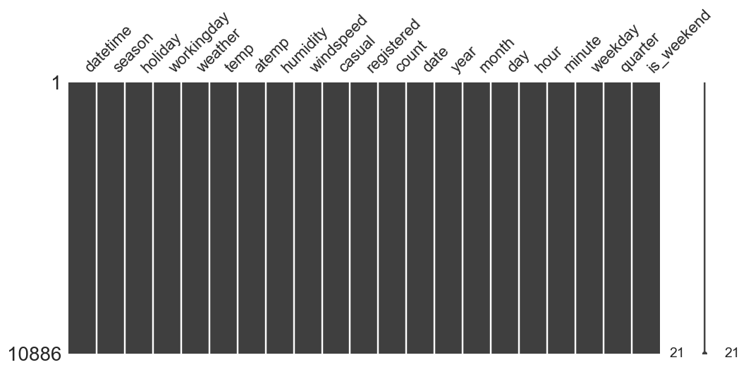
缺失值处理 1 2 12 ,5 ))
<matplotlib.axes._subplots.AxesSubplot at 0x22448f65708>
<class 'pandas.core.frame.DataFrame'>
RangeIndex: 10886 entries, 0 to 10885
Data columns (total 21 columns):
# Column Non-Null Count Dtype
--- ------ -------------- -----
0 datetime 10886 non-null object
1 season 10886 non-null int64
2 holiday 10886 non-null int64
3 workingday 10886 non-null int64
4 weather 10886 non-null int64
5 temp 10886 non-null float64
6 atemp 10886 non-null float64
7 humidity 10886 non-null int64
8 windspeed 10886 non-null float64
9 casual 10886 non-null int64
10 registered 10886 non-null int64
11 count 10886 non-null int64
12 date 10886 non-null datetime64[ns]
13 year 10886 non-null int32
14 month 10886 non-null int32
15 day 10886 non-null int32
16 hour 10886 non-null int32
17 minute 10886 non-null int32
18 weekday 10886 non-null int32
19 quarter 10886 non-null int32
20 is_weekend 10886 non-null int32
dtypes: datetime64[ns](1), float64(3), int32(8), int64(8), object(1)
memory usage: 1.4+ MB
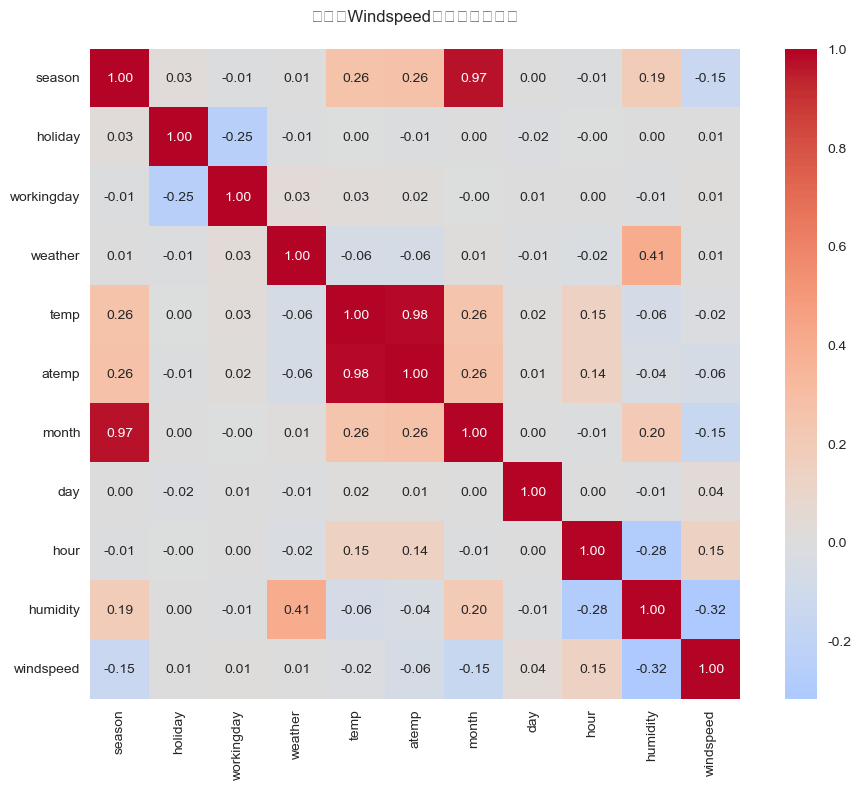
使用随机森林模型预测风速中的0值
1 2 3 4 5 6 7 8 9 10 11 12 13 14 15 16 17 18 19 20 21 22 23 24 25 26 27 28 29 30 31 def analyze_windspeed_correlations (data ):""" 分析特征与windspeed的相关性并绘制热力图 """ 'season' , 'holiday' , 'workingday' , 'weather' , 'temp' , 'atemp' ,'month' ,'day' , 'hour' ,'humidity' , 'windspeed' ]10 , 8 ))True , '.2f' , 'coolwarm' , 0 , True ) '特征与Windspeed的相关性热力图' , pad=20 )'windspeed' ].sort_values(ascending=False )print ("\nWindspeed相关性排序:" )print (correlations)
d:\Development\anaconda3\envs\ml\lib\site-packages\matplotlib\backends\backend_agg.py:211: RuntimeWarning: Glyph 29305 missing from current font.
font.set_text(s, 0.0, flags=flags)
d:\Development\anaconda3\envs\ml\lib\site-packages\matplotlib\backends\backend_agg.py:211: RuntimeWarning: Glyph 24449 missing from current font.
font.set_text(s, 0.0, flags=flags)
d:\Development\anaconda3\envs\ml\lib\site-packages\matplotlib\backends\backend_agg.py:211: RuntimeWarning: Glyph 19982 missing from current font.
font.set_text(s, 0.0, flags=flags)
d:\Development\anaconda3\envs\ml\lib\site-packages\matplotlib\backends\backend_agg.py:211: RuntimeWarning: Glyph 30340 missing from current font.
font.set_text(s, 0.0, flags=flags)
d:\Development\anaconda3\envs\ml\lib\site-packages\matplotlib\backends\backend_agg.py:211: RuntimeWarning: Glyph 30456 missing from current font.
font.set_text(s, 0.0, flags=flags)
d:\Development\anaconda3\envs\ml\lib\site-packages\matplotlib\backends\backend_agg.py:211: RuntimeWarning: Glyph 20851 missing from current font.
font.set_text(s, 0.0, flags=flags)
d:\Development\anaconda3\envs\ml\lib\site-packages\matplotlib\backends\backend_agg.py:211: RuntimeWarning: Glyph 24615 missing from current font.
font.set_text(s, 0.0, flags=flags)
d:\Development\anaconda3\envs\ml\lib\site-packages\matplotlib\backends\backend_agg.py:211: RuntimeWarning: Glyph 28909 missing from current font.
font.set_text(s, 0.0, flags=flags)
d:\Development\anaconda3\envs\ml\lib\site-packages\matplotlib\backends\backend_agg.py:211: RuntimeWarning: Glyph 21147 missing from current font.
font.set_text(s, 0.0, flags=flags)
d:\Development\anaconda3\envs\ml\lib\site-packages\matplotlib\backends\backend_agg.py:211: RuntimeWarning: Glyph 22270 missing from current font.
font.set_text(s, 0.0, flags=flags)
d:\Development\anaconda3\envs\ml\lib\site-packages\matplotlib\backends\backend_agg.py:180: RuntimeWarning: Glyph 29305 missing from current font.
font.set_text(s, 0, flags=flags)
d:\Development\anaconda3\envs\ml\lib\site-packages\matplotlib\backends\backend_agg.py:180: RuntimeWarning: Glyph 24449 missing from current font.
font.set_text(s, 0, flags=flags)
d:\Development\anaconda3\envs\ml\lib\site-packages\matplotlib\backends\backend_agg.py:180: RuntimeWarning: Glyph 19982 missing from current font.
font.set_text(s, 0, flags=flags)
d:\Development\anaconda3\envs\ml\lib\site-packages\matplotlib\backends\backend_agg.py:180: RuntimeWarning: Glyph 30340 missing from current font.
font.set_text(s, 0, flags=flags)
d:\Development\anaconda3\envs\ml\lib\site-packages\matplotlib\backends\backend_agg.py:180: RuntimeWarning: Glyph 30456 missing from current font.
font.set_text(s, 0, flags=flags)
d:\Development\anaconda3\envs\ml\lib\site-packages\matplotlib\backends\backend_agg.py:180: RuntimeWarning: Glyph 20851 missing from current font.
font.set_text(s, 0, flags=flags)
d:\Development\anaconda3\envs\ml\lib\site-packages\matplotlib\backends\backend_agg.py:180: RuntimeWarning: Glyph 24615 missing from current font.
font.set_text(s, 0, flags=flags)
d:\Development\anaconda3\envs\ml\lib\site-packages\matplotlib\backends\backend_agg.py:180: RuntimeWarning: Glyph 28909 missing from current font.
font.set_text(s, 0, flags=flags)
d:\Development\anaconda3\envs\ml\lib\site-packages\matplotlib\backends\backend_agg.py:180: RuntimeWarning: Glyph 21147 missing from current font.
font.set_text(s, 0, flags=flags)
d:\Development\anaconda3\envs\ml\lib\site-packages\matplotlib\backends\backend_agg.py:180: RuntimeWarning: Glyph 22270 missing from current font.
font.set_text(s, 0, flags=flags)
1 2 3 4 5 6 7 8 9 10 11 12 13 14 15 16 17 18 19 20 21 22 23 24 25 26 27 28 29 30 31 32 33 34 35 36 37 38 39 40 41 42 43 44 45 46 47 48 49 50 51 52 53 54 55 56 57 58 59 60 61 62 63 64 65 66 67 68 69 70 71 72 73 74 75 76 77 78 79 80 81 from sklearn.ensemble import RandomForestRegressordef fill_missing_with_rf (data, target_columns, feature_columns=None , missing_value=np.NAN, random_state=42 ):""" 使用随机森林模型填充缺失值 参数: - data: DataFrame, 输入数据 - target_columns: str or list, 需要填充的目标列(可以是单个字符串或列表) - feature_columns: list or None, 用于预测的特征列。如果为None则自动选择数值列 - missing_value: any, 需要填充的值(默认为0)可修改为np.nan # 有bug,缺失值类型无法与target_columns一一匹配 - random_state: int, 随机种子(默认为42) 返回: - DataFrame: 填充后的数据框 """ if isinstance (target_columns, str ):if feature_columns is None :'int64' , 'float64' ]).columnsfor col in feature_columns if col not in target_columns]print (f"自动选择的特征列: {feature_columns} " )for target_column in target_columns:print (f"\n开始处理列: {target_column} " )if target_column not in df.columns:print (f"警告: 列 {target_column} 不存在于数据中" )continue if len (data_missing) == 0 :print (f"列 {target_column} 中没有发现值为{missing_value} 的记录,无需填充。" )continue try :print (f"列 {target_column} 已成功填充 {len (data_missing)} 条记录。" )except Exception as e:print (f"错误: 处理列 {target_column} 时发生异常: {str (e)} " )continue return df'windspeed' , 'humidity' ,'month' ,'season' , 'hour' ,'weather' , 'atemp' ],0 ,42
开始处理列: windspeed
列 windspeed 已成功填充 1313 条记录。
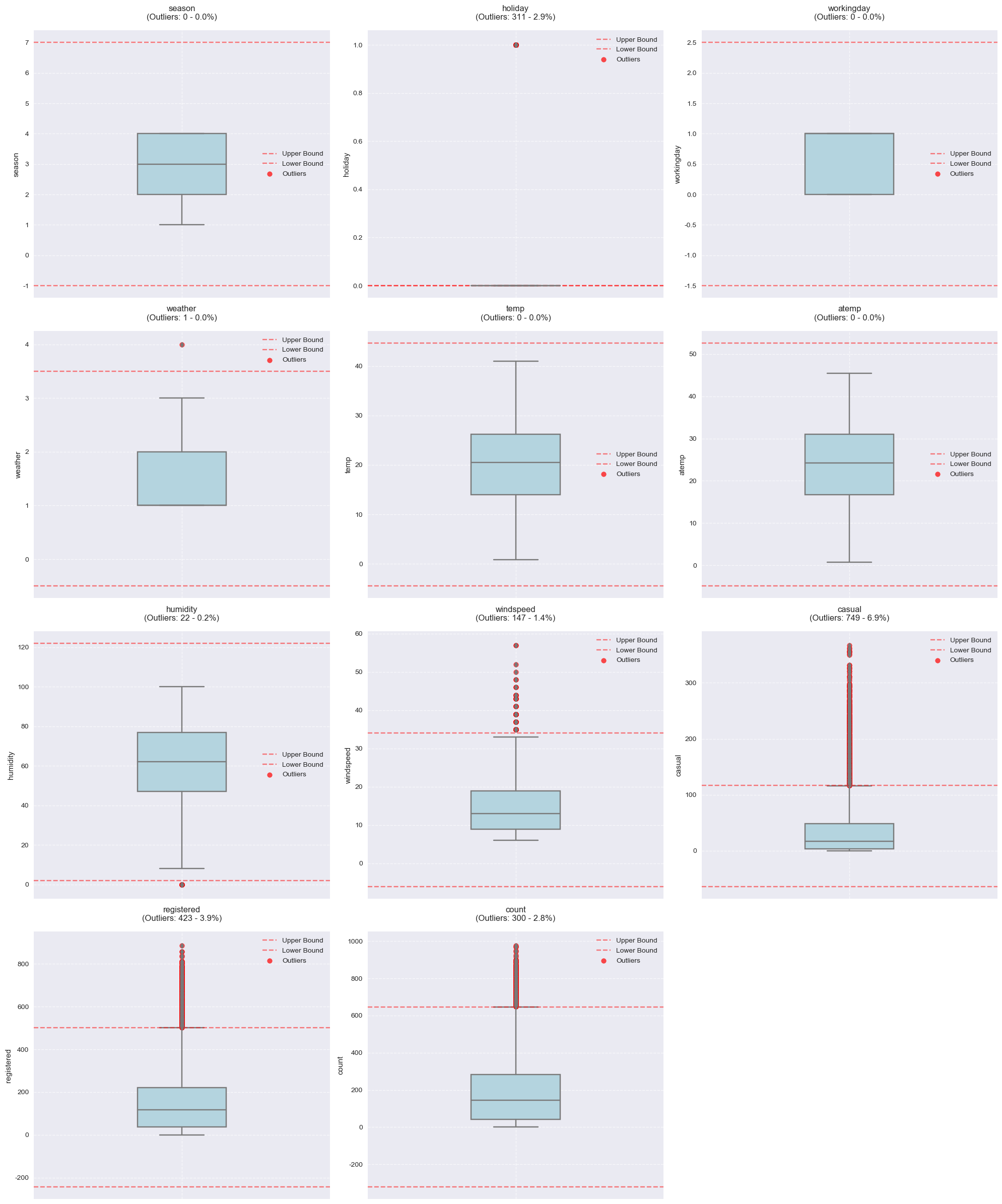
异常值处理 先用IQR检测特征列的异常值,发现humidity和windspeed含有异常值,对于异常值使用季节、温度、天气状况等进行回归插值预测填充。对于目标变量count使用基于模型的方法检测异常值,对异常值进行对数变换 (log transformation) 可以 平滑 count 的分布,减小高值异常值的杠杆效应,使模型更关注相对变化而非绝对变化。
IQR方法检测特征异常值 1 2 3 4 5 6 7 8 9 10 11 12 13 14 15 16 17 18 19 20 21 22 23 24 25 26 27 28 29 30 31 32 33 34 35 36 37 38 39 40 41 42 43 44 45 46 47 48 49 50 51 52 53 54 55 56 57 58 59 60 61 62 63 64 65 66 67 68 69 70 71 72 73 74 75 76 77 78 79 80 81 82 83 84 85 86 87 88 89 90 91 92 93 94 95 96 97 98 99 100 101 102 103 104 105 106 107 108 109 110 111 112 113 114 115 116 117 118 119 120 121 122 123 124 125 126 127 128 129 130 131 132 133 134 135 def plot_iqr_outliers_selected_columns (data, columns=None , threshold=1.5 ):""" 使用IQR方法检测并可视化指定列的异常值 参数: - data: DataFrame, 输入数据 - columns: list or None, 需要检测的列名列表。如果为None,则检测所有数值列 - threshold: float, IQR的倍数阈值,默认为1.5 返回: - outliers_summary: dict, 异常值检测结果摘要 """ if columns is None :'int64' , 'float64' ]).columnselse :for col in columns:if col not in data.columns:raise ValueError(f"列 '{col} ' 不存在于数据中" )if not np.issubdtype(data[col].dtype, np.number):raise ValueError(f"列 '{col} ' 不是数值类型" )0.25 )0.75 )print (f"\n{'=' *20 } IQR异常值检测报告 {'=' *20 } " )for column in columns:len (outliers)len (data))*100 'Q1' : Q1[column],'Q3' : Q3[column],'IQR' : IQR[column],'lower_bound' : lower_bounds[column],'upper_bound' : upper_bounds[column],'outliers_count' : outliers_count,'outliers_percentage' : outliers_percentage,'outliers_index' : outliers_idx, 'outliers_values' : data.loc[outliers_idx, column] print (f"\n列名: {column} " )print (f"Q1: {Q1[column]:.2 f} " )print (f"Q3: {Q3[column]:.2 f} " )print (f"IQR: {IQR[column]:.2 f} " )print (f"下界: {lower_bounds[column]:.2 f} " )print (f"上界: {upper_bounds[column]:.2 f} " )print (f"异常值数量: {outliers_count} " )print (f"异常值占比: {outliers_percentage:.2 f} %" )min (3 , len (columns))len (columns) + n_cols - 1 ) // n_cols'seaborn' )20 , 6 *n_rows))if n_rows * n_cols > 1 else [axes]for idx, column in enumerate (columns):'outliers_index' ]'lightblue' , width=0.3 )len (outliers_idx)), 'red' , alpha=0.7 , label='Outliers' 'r' , linestyle='--' , 0.5 , label='Upper Bound' 'r' , linestyle='--' , 0.5 , label='Lower Bound' f'{column} \n(Outliers: {outliers_summary[column]["outliers_count" ]} - ' f'{outliers_summary[column]["outliers_percentage" ]:.1 f} %)' , 15 True , linestyle='--' , alpha=0.7 )for idx in range (len (columns), len (axes)):return outliers_summary
==================== IQR异常值检测报告 ====================
列名: season
Q1: 2.00
Q3: 4.00
IQR: 2.00
下界: -1.00
上界: 7.00
异常值数量: 0
异常值占比: 0.00%
列名: holiday
Q1: 0.00
Q3: 0.00
IQR: 0.00
下界: 0.00
上界: 0.00
异常值数量: 311
异常值占比: 2.86%
列名: workingday
Q1: 0.00
Q3: 1.00
IQR: 1.00
下界: -1.50
上界: 2.50
异常值数量: 0
异常值占比: 0.00%
列名: weather
Q1: 1.00
Q3: 2.00
IQR: 1.00
下界: -0.50
上界: 3.50
异常值数量: 1
异常值占比: 0.01%
列名: temp
Q1: 13.94
Q3: 26.24
IQR: 12.30
下界: -4.51
上界: 44.69
异常值数量: 0
异常值占比: 0.00%
列名: atemp
Q1: 16.66
Q3: 31.06
IQR: 14.39
下界: -4.93
上界: 52.65
异常值数量: 0
异常值占比: 0.00%
列名: humidity
Q1: 47.00
Q3: 77.00
IQR: 30.00
下界: 2.00
上界: 122.00
异常值数量: 22
异常值占比: 0.20%
列名: windspeed
Q1: 9.00
Q3: 19.00
IQR: 10.00
下界: -6.01
上界: 34.01
异常值数量: 147
异常值占比: 1.35%
列名: casual
Q1: 4.00
Q3: 49.00
IQR: 45.00
下界: -63.50
上界: 116.50
异常值数量: 749
异常值占比: 6.88%
列名: registered
Q1: 36.00
Q3: 222.00
IQR: 186.00
下界: -243.00
上界: 501.00
异常值数量: 423
异常值占比: 3.89%
列名: count
Q1: 42.00
Q3: 284.00
IQR: 242.00
下界: -321.00
上界: 647.00
异常值数量: 300
异常值占比: 2.76%
1 2 3 4 5 6 7 8 9 10 11 12 13 14 15 16 17 18 19 20 21 22 23 24 25 26 27 28 29 30 31 32 33 34 35 36 37 38 39 40 41 42 43 44 45 46 47 48 49 50 51 52 53 54 55 56 57 58 59 60 61 62 63 64 65 66 67 68 69 70 import osdef get_column_outliers (outliers_summary, column_name, data, save_csv=True , output_dir='./outliers' ):""" 获取指定列的异常值详情,并可选择保存完整样本数据为CSV文件 参数: - outliers_summary: dict, 异常值检测结果字典 - column_name: str, 列名 - data: DataFrame, 原始数据集 - save_csv: bool, 是否保存为CSV文件,默认为True - output_dir: str, CSV文件输出目录,默认为'./outliers' 返回: - DataFrame: 包含异常值的完整样本数据 """ if column_name not in outliers_summary:raise ValueError(f"列 '{column_name} ' 不在异常值检测结果中" )print (f"\n{'=' *20 } {column_name} 异常值详情 {'=' *20 } " )print (f"异常值数量: {outliers_info['outliers_count' ]} " )print (f"异常值占比: {outliers_info['outliers_percentage' ]:.2 f} %" )print (f"\n异常值分布:" )print (f"最小值: {outliers_info['outliers_values' ].min ():.2 f} " )print (f"最大值: {outliers_info['outliers_values' ].max ():.2 f} " )print (f"均值: {outliers_info['outliers_values' ].mean():.2 f} " )print (f"标准差: {outliers_info['outliers_values' ].std():.2 f} " )'outliers_index' ]].copy()'is_outlier' ] = True 'outlier_value' ] = outliers_info['outliers_values' ]if save_csv:if not os.path.exists(output_dir):print (f"\n创建输出目录: {output_dir} " )'%Y%m%d_%H%M%S' )f"{column_name} _outliers_samples_{timestamp} .csv" True , encoding='utf-8' )print (f"\n异常值完整样本数据已保存至: {filepath} " )return outliers_data'humidity' , 'windspeed' ]for column in selected_columns_detail:print ("\n" )True , './outliers' print ("\n异常值样本预览:" )
异常值分布:
最小值: 0.00
最大值: 0.00
均值: 0.00
标准差: 0.00
异常值完整样本数据已保存至: ./outliers\humidity_outliers_samples_20250224_181014.csv
异常值样本预览:
datetime
season
holiday
workingday
weather
temp
atemp
humidity
windspeed
casual
...
year
month
day
hour
minute
weekday
quarter
is_weekend
is_outlier
outlier_value
1091
2011-03-10 00:00:00
1
0
1
3
13.94
15.910
0
16.9979
3
...
2011
3
10
0
0
3
1
0
True
0
1092
2011-03-10 01:00:00
1
0
1
3
13.94
15.910
0
16.9979
0
...
2011
3
10
1
0
3
1
0
True
0
1093
2011-03-10 02:00:00
1
0
1
3
13.94
15.910
0
16.9979
0
...
2011
3
10
2
0
3
1
0
True
0
1094
2011-03-10 05:00:00
1
0
1
3
14.76
17.425
0
12.9980
1
...
2011
3
10
5
0
3
1
0
True
0
1095
2011-03-10 06:00:00
1
0
1
3
14.76
16.665
0
22.0028
0
...
2011
3
10
6
0
3
1
0
True
0
5 rows × 23 columns
异常值分布:
最小值: 35.00
最大值: 57.00
均值: 38.54
标准差: 4.27
异常值完整样本数据已保存至: ./outliers\windspeed_outliers_samples_20250224_181015.csv
异常值样本预览:
datetime
season
holiday
workingday
weather
temp
atemp
humidity
windspeed
casual
...
year
month
day
hour
minute
weekday
quarter
is_weekend
is_outlier
outlier_value
178
2011-01-08 17:00:00
1
0
0
1
6.56
6.060
37
36.9974
5
...
2011
1
8
17
0
5
1
1
True
36.9974
194
2011-01-09 09:00:00
1
0
0
1
4.92
3.790
46
35.0008
0
...
2011
1
9
9
0
6
1
1
True
35.0008
196
2011-01-09 11:00:00
1
0
0
1
6.56
6.060
40
35.0008
2
...
2011
1
9
11
0
6
1
1
True
35.0008
265
2011-01-12 12:00:00
1
0
1
1
8.20
7.575
47
39.0007
3
...
2011
1
12
12
0
2
1
0
True
39.0007
271
2011-01-12 18:00:00
1
0
1
1
8.20
7.575
47
35.0008
2
...
2011
1
12
18
0
2
1
0
True
35.0008
5 rows × 23 columns
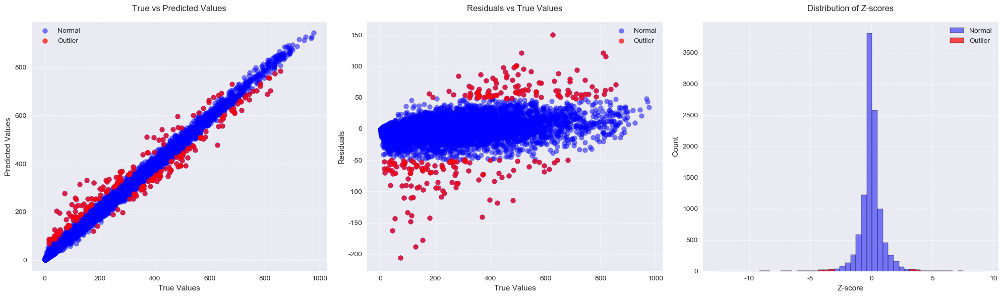
基于模型检测目标变量异常值 代码整体思路:
通过计算模型预测值和真实y值之间的残差,并利用残差的均值和标准差来计算z值。然后,根据设定的sigma阈值,将绝对值大于sigma的z值作为异常值进行检测和标记。最后,通过打印输出和可视化子图展示异常值的相关信息。目的是识别和理解模型中的异常值,以便进一步进行数据处理或模型调整。
1 2 3 4 5 6 7 8 9 10 11 12 13 14 15 16 17 18 19 20 21 22 23 24 25 26 27 28 29 30 31 32 33 34 35 36 37 38 39 40 41 42 43 44 45 46 47 48 49 50 51 52 53 54 55 56 57 58 59 60 61 62 63 64 65 66 67 68 69 70 71 72 73 74 75 76 77 78 79 80 81 82 83 84 85 86 87 88 89 90 91 92 93 94 95 96 97 98 99 100 101 102 103 104 105 106 107 108 109 110 111 112 113 114 115 116 117 118 119 120 from sklearn.metrics import mean_squared_errordef rmse (y_true, y_pred ):"""均方根误差""" return np.sqrt(mean_squared_error(y_true, y_pred))def find_outliers (model, data, feature_columns, target='count' , sigma=3 ):""" 检测数据集中的异常值。 参数: - model: 用于预测的模型对象 - data: DataFrame, 包含特征和目标变量的数据集 - feature_columns: list, 用于预测的特征列名列表 - target: str, 目标变量列名,默认为'count' - sigma: float, 标准差倍数阈值,默认为3 返回: - outliers: 异常值的索引 """ try :except :abs (z) > sigma].indexprint (f"\n{'=' *20 } 异常值检测报告 {'=' *20 } " )print ("\n1. 模型性能指标:" )print (f"R² score: {model.score(X,y):.4 f} " )print (f"RMSE: {rmse(y, y_pred):.4 f} " )print (f"MSE: {mean_squared_error(y,y_pred):.4 f} " )print ("\n2. 残差统计信息:" )print (f"残差均值: {mean_resid:.4 f} " )print (f"残差标准差: {std_resid:.4 f} " )print ("\n3. 异常值统计:" )print (f"检测到的异常值数量: {len (outliers)} " )print (f"异常值占比: {(len (outliers)/len (data))*100 :.2 f} %" )'seaborn' )1 , 3 , figsize=(20 , 6 ))0 ].scatter(y, y_pred, c='blue' , alpha=0.5 , label='Normal' )0 ].scatter(y.loc[outliers], y_pred.loc[outliers], 'red' , alpha=0.7 , label='Outlier' )0 ].set_title('True vs Predicted Values' , pad=15 )0 ].set_xlabel('True Values' )0 ].set_ylabel('Predicted Values' )0 ].legend()0 ].grid(True , linestyle='--' , alpha=0.7 )1 ].scatter(y, y-y_pred, c='blue' , alpha=0.5 , label='Normal' )1 ].scatter(y.loc[outliers], y.loc[outliers]-y_pred.loc[outliers], 'red' , alpha=0.7 , label='Outlier' )1 ].set_title('Residuals vs True Values' , pad=15 )1 ].set_xlabel('True Values' )1 ].set_ylabel('Residuals' )1 ].legend()1 ].grid(True , linestyle='--' , alpha=0.7 )50 , ax=axes[2 ], color='blue' , 0.5 , label='Normal' )50 , ax=axes[2 ], 'red' , alpha=0.7 , label='Outlier' )2 ].set_title('Distribution of Z-scores' , pad=15 )2 ].set_xlabel('Z-score' )2 ].set_ylabel('Count' )2 ].legend()2 ].grid(True , linestyle='--' , alpha=0.7 )return outliers'season' , 'weather' , 'temp' , 'atemp' , 'humidity' , 'windspeed' , 'year' , 'month' , 'hour' , 'weekday' 100 , random_state=42 )'count' ,3
==================== 异常值检测报告 ====================
1. 模型性能指标:
R² score: 0.9920
RMSE: 16.2065
MSE: 262.6518
2. 残差统计信息:
残差均值: -0.5107
残差标准差: 16.1992
3. 异常值统计:
检测到的异常值数量: 213
异常值占比: 1.96%
1 train_data.loc[outliers]
datetime
season
holiday
workingday
weather
temp
atemp
humidity
windspeed
casual
...
count
date
year
month
day
hour
minute
weekday
quarter
is_weekend
380
2011-01-17 08:00:00
1
1
0
2
6.56
7.575
47
15.001300
3
...
33
2011-01-17
2011
1
17
8
0
0
1
0
1699
2011-04-16 17:00:00
2
0
0
3
20.50
24.240
88
39.000700
1
...
15
2011-04-16
2011
4
16
17
0
5
2
1
1802
2011-05-02 00:00:00
2
0
1
1
18.86
22.725
72
8.998100
68
...
177
2011-05-02
2011
5
2
0
0
0
2
0
2035
2011-05-11 17:00:00
2
0
1
1
26.24
31.060
47
7.001500
17
...
259
2011-05-11
2011
5
11
17
0
2
2
0
2036
2011-05-11 18:00:00
2
0
1
1
25.42
31.060
50
19.999500
40
...
274
2011-05-11
2011
5
11
18
0
2
2
0
...
...
...
...
...
...
...
...
...
...
...
...
...
...
...
...
...
...
...
...
...
...
10271
2012-11-13 09:00:00
4
0
1
3
13.12
15.150
81
22.002800
1
...
110
2012-11-13
2012
11
13
9
0
1
4
0
10466
2012-12-02 12:00:00
4
0
0
2
13.94
16.665
81
11.001400
111
...
520
2012-12-02
2012
12
2
12
0
6
4
1
10486
2012-12-03 08:00:00
4
0
1
1
14.76
18.940
93
7.776656
19
...
731
2012-12-03
2012
12
3
8
0
0
4
0
10533
2012-12-05 07:00:00
4
0
1
3
18.86
22.725
59
19.999500
9
...
398
2012-12-05
2012
12
5
7
0
2
4
0
10582
2012-12-07 08:00:00
4
0
1
2
12.30
14.395
75
12.998000
11
...
441
2012-12-07
2012
12
7
8
0
4
4
0
213 rows × 21 columns
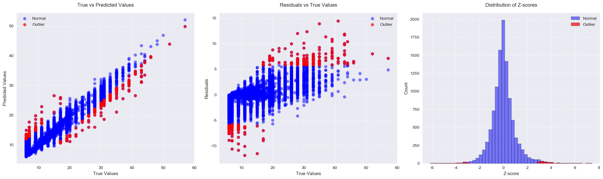
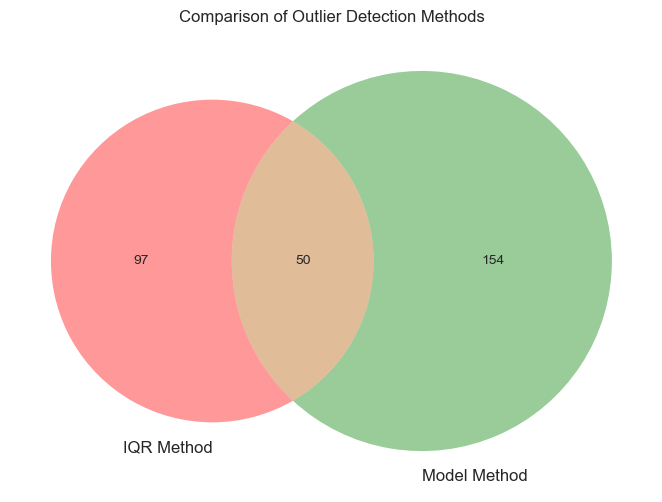
IQR与模型方法对比分析 1 2 3 4 5 6 7 8 9 10 11 12 13 14 15 16 17 18 19 20 21 22 23 24 25 26 27 28 29 30 31 32 33 34 35 36 37 38 39 40 41 42 43 44 45 46 47 48 49 50 51 52 53 54 55 56 57 58 59 60 61 62 63 64 65 66 67 68 69 from matplotlib_venn import venn2'font.sans-serif' ] = ['SimHei' ] 'axes.unicode_minus' ] = False def compare_outlier_methods (data, feature_columns, target='count' , iqr_threshold=1.5 , model_sigma=3 ):""" 比较IQR方法和基于模型的异常值检测方法 参数: - data: DataFrame, 输入数据 - feature_columns: list, 用于检测target变量的特征 - target: str, 待检测变量列名 - iqr_threshold: float, IQR方法的阈值 - model_sigma: float, 模型方法的sigma阈值 """ 0.25 )0.75 )100 , random_state=42 )print ("\n比较结果:" )print (f"IQR方法检测到的异常值数量: {len (iqr_outliers)} " )print (f"模型方法检测到的异常值数量: {len (model_outliers)} " )set (iqr_outliers) & set (model_outliers)print (f"两种方法共同检测到的异常值数量: {len (common_outliers)} " )12 , 6 ))set (iqr_outliers), set (model_outliers)], 'IQR Method' , 'Model Method' ))'Comparison of Outlier Detection Methods' )return {'iqr_outliers' : iqr_outliers,'model_outliers' : model_outliers,'common_outliers' : common_outliers'season' , 'weather' , 'temp' , 'atemp' , 'humidity' , 'year' , 'month' , 'hour' 'windspeed' ,1.5 ,3
==================== 异常值检测报告 ====================
1. 模型性能指标:
R² score: 0.9188
RMSE: 1.9433
MSE: 3.7765
2. 残差统计信息:
残差均值: -0.0311
残差标准差: 1.9432
3. 异常值统计:
检测到的异常值数量: 204
异常值占比: 1.87%
1 2 3 4 5 6 7 8 9 10 11 12 13 14 15 16 17 18 19 20 21 22 23 24 25 26 27 28 29 30 31 32 33 34 35 36 37 38 39 40 41 42 43 44 45 46 "IQR方法" : {"优点" : ["无需模型训练,计算简单快速" ,"基于数据分布特征,不受模型影响" ,"适用于单变量分析" ,"容易理解和解释" ,"对数据分布假设较少" "缺点" : ["无法考虑特征之间的关系" ,"可能忽略多维数据中的复杂异常模式" ,"对多变量异常值检测效果不佳" ,"固定的阈值(1.5*IQR)可能不适合所有场景" "适用场景" : ["数据预处理初期的快速异常检测" ,"单变量异常值分析" ,"数据分布较为对称的情况" ,"需要快速获得数据质量概览" "基于模型的方法(find_outliers)" : {"优点" : ["考虑了特征间的相互关系" ,"可以发现复杂的异常模式" ,"基于预测残差,更符合业务逻辑" ,"可以根据模型预测效果动态调整" ,"适合处理多维特征的异常值" "缺点" : ["需要训练模型,计算成本较高" ,"依赖模型的质量和选择" ,"可能受到模型过拟合的影响" ,"参数调整较为复杂" "适用场景" : ["多变量异常值检测" ,"需要考虑特征关联性的场景" ,"有明确的预测目标" ,"数据量较大且特征较多的情况"
建议:
对于自行车租赁需求预测这个场景,我建议使用基
需求预测涉及多个特征的交互作用
异常值可能与多个因素相关(如天气、温度、时间等)
预测目标明确,适合使用模型方法
数据量较大,特征较多
最佳实践:
可以先用IQR方法进行初步筛查
再使用模型方法进行深入分析
重点关注两种方法都检测出的异常值
结合业务逻辑判断是否需要处理这些异常值
处理建议:
对于共同检测出的异常值,优先考虑处理
仅被单个方法检测出的异常值需要进一步分析
结合业务场景判断是否为真实异常
可以考虑对异常值进行分类处理而不是简单删除
参数调整:
主要区别:
IQR方法(plot_iqr_outliers_all_columns):
检测所有数值列的异常值
基于每列自身的分布特征(Q1, Q3, IQR)
不考虑特征之间的关系
适合单变量分析
基于模型的方法(find_outliers):
只检测目标变量 ‘count’ 的异常值
基于所有特征列预测 ‘count’ 的结果
考虑了特征与目标变量之间的关系
适合多变量分析
这个改进版本的主要特点:
迭代处理:
每轮迭代先处理特征列的异常值
再检测目标变量的异常值
合并两种方法检测到的异常值
双重检测:
使用IQR方法检测特征列异常值
使用基于模型的方法检测目标变量异常值
异常值处理:
使用中位数替换检测到的异常值
下一轮迭代使用处理后的数据继续检测
终止条件:
结果可视化:
展示每轮迭代检测到的异常值数量
帮助理解异常值检测的收敛过程
这种方法的优势:
更全面:同时考虑特征列和目标变量的异常值
更稳健:通过迭代方式逐步处理异常值
更可靠:结合多种检测方法,互相验证
可追踪:记录每轮迭代的检测结果
使用建议:
根据数据特点调整 $sigma$ 和 $max_iterations$ 参数
观察迭代过程中异常值数量的变化
结合业务逻辑判断是否需要处理所有检测到的异常值
可以尝试不同的异常值替换方法(如均值、插值等)
异常值处理策略 outlier_handling_methods = {
"2. 删除异常值": {
"方法描述": [
"直接删除被识别为异常的样本",
"清理数据集",
"适用于异常值明显错误的场景"
],
"优点": [
"处理方法简单直接",
"可以提高数据质量",
"减少噪声影响"
],
"缺点": [
"可能丢失有用信息",
"减少样本量",
"可能引入选择偏差"
],
"适用性评分": "低",
"适用场景": [
"异常值明显是错误数据",
"样本量充足",
"异常值比例较小"
]
},
"3. 替换异常值": {
"统计替换": {
"方法描述": [
"使用统计量替换异常值",
"常用统计量:均值、中位数、众数",
"可以按分组进行替换"
],
"优点": [
"实现简单",
"保持数据量",
"不改变整体分布"
],
"缺点": [
"可能降低数据方差",
"可能忽略特征关系",
"替换值可能不符合实际"
],
"适用性评分": "中等",
"适用场景": [
"异常值分布较随机",
"特征间相关性不强",
"需要快速处理"
]
},
"插值替换": {
"方法描述": [
"使用相邻值进行插值",
"可以是线性插值或更复杂的插值方法",
"考虑数据的时间序列特性"
],
"优点": [
"保持数据的连续性",
"考虑时间序列特征",
"更符合实际变化"
],
"缺点": [
"计算复杂度较高",
"需要合适的时间窗口",
"可能受噪声影响"
],
"适用性评分": "高",
"适用场景": [
"时间序列数据",
"数据具有连续性",
"异常值周围有可靠数据"
]
},
"模型预测替换": {
"方法描述": [
"使用模型预测值替换异常值",
"可以考虑多个特征的关系",
"适合复杂的数据关系"
],
"优点": [
"考虑特征间关系",
"预测值更准确",
"适应性强"
],
"缺点": [
"计算成本高",
"依赖模型质量",
"可能过度平滑"
],
"适用性评分": "高",
"适用场景": [
"特征间有强相关性",
"有足够训练数据",
"需要高精度替换"
]
}
},
"4. 分箱处理": {
"方法描述": [
"将异常值映射到合适的分箱中",
"可以是等宽分箱或等频分箱",
"处理极端值"
],
"优点": [
"保持数据的相对关系",
"减少极端值影响",
"便于特征工程"
],
"缺点": [
"损失精确信息",
"需要合理的分箱策略",
"可能影响预测精度"
],
"适用性评分": "中等",
"适用场景": [
"处理极端值",
"特征工程需要",
"类别化处理"
]
}
}
针对自行车租赁需求预测项目的建议处理方案:
数据集成 数据重采样 数据变换- 连续变量离散化 (分箱) 数据变换- 长尾分布处理 长尾分布更多出现在以下两类场景中:
多类别场景的类别分布:
某一离散特征的取值分布:
偏度调整
根据直方图和Q-Q图考虑是否对数据进行变换,使之符合正态分布
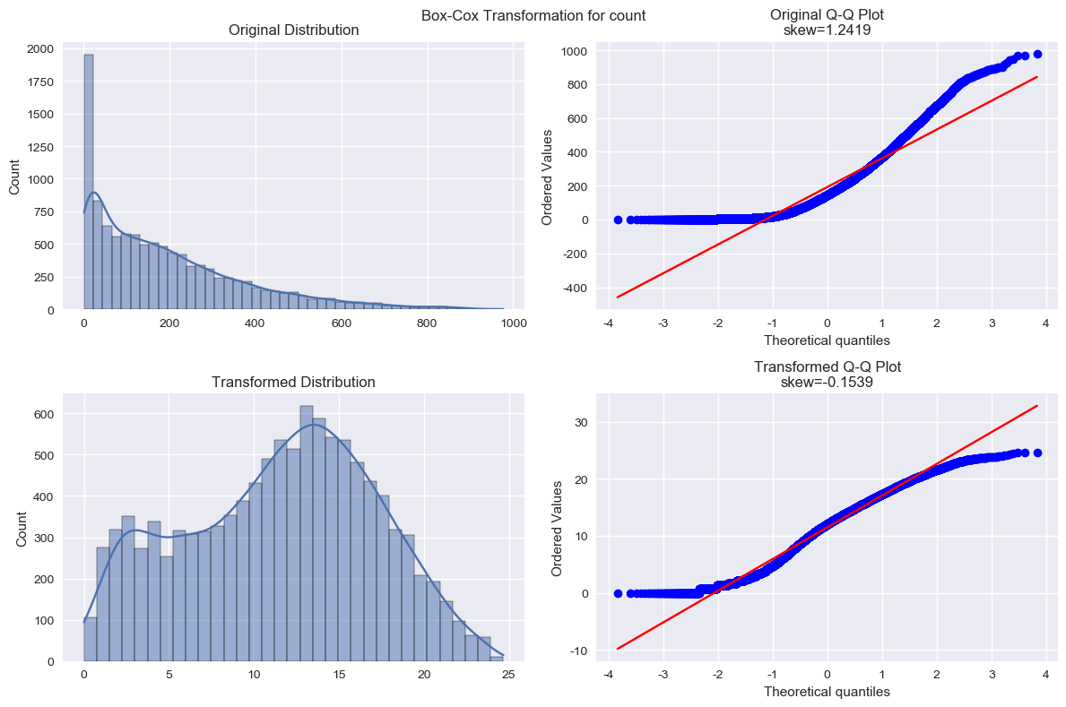
Box-Cox变换
Box-Cox 变换是一种常见的数据转换技术,用于将非正态分布的数据转换为近似正态分布 的数据。这一变换可以使线性回归模型在满足线性、正态性、独立性及方差齐性的同时,又不丢失信息。在对数据做Box-Cox变换之后,可以在一定程度上减小不可观测的误差和预测变量的相关性,这有利于线性模型的拟合及分析出特征的相关性 。
先归一化还是先转换?
在做Box-Cox变换之前,需要对数据做归一化预处理。在归一化时,对数据进行合并操作可以使训练数据和测试数据一致。这种方式可以在线下分析建模中使用,而线上部署只需采用训练数据的归一化即可。
1.一般情况下,先Box-Cox后归一化
2.有负值时,考虑先归一化后Box-Cox
3.还原时顺序要与转换顺序相反
4.建议先检查数据特征再决定处理顺序
5.保持转换顶序的一致性和可追踪性
对特征变量进行转换吗?
是否需要对特征变量和目标变量都进行转换,取决于数据的分布、模型的要求以及你希望达成的目标。通常情况下,对目标变量进行转换更为常见,因为这有助于满足许多统计模型的假设。但是,在某些情况下,对特征变量进行转换也是有益的。最佳做法是尝试不同的转换方法,并根据模型的性能进行选择。
Box-Cox转换 = {
1 2 3 4 5 6 7 8 9 10 11 12 13 14 15 16 17 18 19 20 21 22 23 24 25 26 27 28 29 30 31 32 33 34 35 36 37 38 39 40 41 42 43 44 45 46 47 48 49 50 51 52 53 54 55 56 57 58 59 60 61 62 63 64 65 66 67 68 69 70 71 72 73 74 75 76 77 78 79 80 81 82 83 84 85 86 87 88 89 90 91 92 93 94 95 96 97 98 99 100 101 102 103 104 105 106 107 108 109 110 111 112 113 114 115 116 117 118 119 120 121 122 123 124 125 126 127 128 129 130 131 132 133 134 135 136 137 138 139 140 141 142 143 144 145 146 147 148 149 150 151 152 153 154 155 156 157 158 159 160 161 162 163 164 165 166 167 168 169 170 171 172 173 174 175 176 177 178 179 180 181 182 183 184 185 186 187 188 189 190 191 192 193 194 195 196 197 198 199 200 201 202 203 204 205 206 207 208 209 210 211 212 213 214 215 216 217 218 219 220 221 222 223 224 225 226 class BoxCoxPipeline :""" Box-Cox转换通用流程 支持: 1. 同时转换特征列和目标变量列 2. 对测试集进行相同的转换 3. 智能处理测试集中不存在的目标变量列 1. 支持同时转换特征列和目标变量: * 通过`columns`参数指定特征列 * 通过`target_col`参数指定目标变量 * 内部分别存储特征列和目标变量信息 2. 测试集转换: * `transform`方法会自动检查哪些列存在于测试集中 * 只对存在的列进行转换 * 提供警告信息说明转换了哪些列 3. 处理测试集中不存在的目标变量列: * `transform`方法会跳过不存在的列 * `inverse_transform`方法默认还原目标变量 * 可以通过`columns`参数指定要还原的列 """ def __init__ (self, visualization=False ):self .lambda_params = {} self .shifts = {} self .visualization = visualizationself .transformed_columns = None self .feature_columns = None self .target_column = None def _get_numeric_columns (self, data ):"""获取数值型列名""" return data.select_dtypes(include=['int64' , 'float64' ]).columns.tolist()def _handle_non_positive (self, x ):"""处理非正值""" min ()if min_val <= 0 :abs (min_val) + 1 return x + shift, shiftreturn x, 0 def _plot_transformation (self, original, transformed, col_name ):"""可视化转换效果""" 2 , 2 , figsize=(12 , 8 ))f'Box-Cox Transformation for {col_name} ' )0 ,0 ], kde=True )0 ,0 ].set_title('Original Distribution' )0 ,1 ])0 ,1 ].set_title(f'Original Q-Q Plot\nskew={stats.skew(original):.4 f} ' )1 ,0 ], kde=True )1 ,0 ].set_title('Transformed Distribution' )1 ,1 ])1 ,1 ].set_title(f'Transformed Q-Q Plot\nskew={stats.skew(transformed):.4 f} ' )def fit_transform (self, data, columns=None , target_col=None ):""" 拟合并转换数据 参数: - data: DataFrame, 输入数据 - columns: list or str, 需要转换的特征列名列表或单个列名 - target_col: str, 目标变量列名 返回: - DataFrame: 转换后的数据 """ if columns is not None :if isinstance (columns, str ) else list (columns)if target_col else [])for col in all_cols:if col not in data.columns:raise ValueError(f"列 {col} 不存在于数据中" )if col not in self ._get_numeric_columns(data):raise ValueError(f"列 {col} 不是数值型" )self .feature_columns = feature_colsself .target_column = target_colself .transformed_columns = all_colsprint (f"将进行以下转换:" )if feature_cols:print (f"- 特征列: {feature_cols} " )if target_col:print (f"- 目标变量: {target_col} " )for col in self .transformed_columns:try :self ._handle_non_positive(data[col].values)self .shifts[col] = shiftself .lambda_params[col] = lambda_paramprint (f"\n列 {col} 转换结果:" )print (f"- Lambda参数: {lambda_param:.4 f} " )print (f"- 偏移量: {shift} " )print (f"- 偏度变化: {stats.skew(data[col]):.4 f} -> {stats.skew(transformed_x):.4 f} " )if self .visualization:self ._plot_transformation(data[col].values, transformed_x, col)except Exception as e:print (f"警告: 列 {col} 转换失败: {str (e)} " )continue return resultdef transform (self, data ):""" 使用已有参数转换新数据 参数: - data: DataFrame, 需要转换的数据 返回: - DataFrame: 转换后的数据 """ if not self .lambda_params:raise ValueError("请先调用fit_transform" )for col in self .transformed_columns if col in data.columns]if not columns_to_transform:print ("警告: 没有需要转换的列" )return resultprint (f"对以下列进行转换: {columns_to_transform} " )for col in columns_to_transform:self .shifts[col]self .lambda_params[col]if lambda_param == 0 :else :1 ) / lambda_paramreturn resultdef inverse_transform (self, data, columns=None ):""" 逆转换回原始尺度 参数: - data: DataFrame或array-like, 需要还原的数据 - columns: list or str, 需要还原的列名(如果data是DataFrame) 如果data是array-like且未指定columns,默认还原目标变量 返回: - DataFrame或array: 还原后的数据 """ if not self .lambda_params:raise ValueError("请先调用fit_transform" )if isinstance (data, (pd.Series, list , np.ndarray)):if columns is None :if self .target_column:self .target_columnelif len (self .transformed_columns) == 1 :self .transformed_columns[0 ]else :raise ValueError("无法确定要还原的列,请指定columns参数" )else :0 ] if isinstance (columns, list ) else columnsif self .lambda_params[col] == 0 :else :self .lambda_params[col] * x + 1 , 1 /self .lambda_params[col])self .shifts[col], 0 )return restoredor self .transformed_columnsfor col in columns_to_restore:if col not in self .lambda_params or col not in data.columns:continue self .lambda_params[col]if lambda_param == 0 :else :1 , 1 /lambda_param)self .shifts[col], 0 )return result
1 2 3 4 5 6 7 8 9 10 11 12 13 14 15 16 True )'count'
将进行以下转换:
- 目标变量: count
列 count 转换结果:
- Lambda参数: 0.3157
- 偏移量: 0
- 偏度变化: 1.2419 -> -0.1539
3.2 特征构造 特征组合: 将多个特征进行组合,例如加减乘除、交叉组合等,以创建新的特征。
多项式特征: 创建原始特征的多项式组合,例如平方、立方等。
基于业务逻辑的特征: 根据业务逻辑和领域知识,设计新的特征。例如,在电商场景中,可以构建“最近一个月购买次数”等特征。
1 2 3 4 5 6 7 8 9 10 11 12 13 14 15 16 17 18 19 20 21 22 23 24 25 26 27 28 29 30 31 32 33 34 35 36 37 38 39 40 41 42 43 44 45 46 47 48 49 50 51 52 53 54 55 56 57 58 59 60 61 62 63 64 65 66 67 68 69 70 71 72 73 74 75 76 77 78 79 80 81 82 83 84 85 86 87 88 89 90 91 92 93 94 95 96 97 98 99 100 101 102 103 104 105 106 107 108 109 110 111 112 113 114 115 116 117 118 119 120 121 122 123 124 125 126 127 128 129 130 131 132 133 134 135 136 137 138 139 140 141 142 143 144 145 146 147 148 149 150 151 152 153 154 155 156 157 158 159 160 161 162 163 164 165 166 167 168 169 170 171 172 173 174 175 176 177 178 179 180 181 182 183 184 185 186 187 188 189 190 191 192 193 194 195 196 197 198 199 200 201 202 203 204 205 206 207 208 209 210 211 212 213 214 215 216 217 218 219 220 221 222 223 224 225 226 227 228 229 230 231 232 233 234 235 236 237 238 239 240 241 242 243 244 245 246 247 248 249 250 251 252 253 254 255 256 257 258 259 260 261 262 263 264 265 266 267 268 269 270 271 272 273 274 275 276 277 278 279 280 281 282 283 284 285 286 287 288 289 290 291 292 293 294 295 296 297 import numpy as npimport pandas as pdfrom sklearn.preprocessing import LabelEncoder, StandardScalerfrom sklearn.base import BaseEstimator, TransformerMixinclass BikeShareFeatureEngineering (BaseEstimator, TransformerMixin):"""自行车共享系统的特征工程类""" def __init__ (self ):self .scaler = StandardScaler()self .label_encoders = {}def fit (self, X, y=None ):return self def transform (self, df ):"""转换数据""" self ._create_time_features(df)self ._process_weather_features(df)self ._process_temperature_features(df)self ._create_interaction_features(df)self ._select_features(df)return dfdef _create_time_features (self, df ):"""创建时间特征""" 'datetime' ] = pd.to_datetime(df['datetime' ])'dayofweek' ] = df['datetime' ].dt.dayofweek'hour_sin' ] = np.sin(2 * np.pi * df['hour' ]/24 )'hour_cos' ] = np.cos(2 * np.pi * df['hour' ]/24 )'month_sin' ] = np.sin(2 * np.pi * (df['month' ]-1 )/12 )'month_cos' ] = np.cos(2 * np.pi * (df['month' ]-1 )/12 )'workday_hour' ] = df['hour' ] * df['workingday' ]'weekend_hour' ] = df['hour' ] * (1 - df['workingday' ])'rush_hour' ] = ((df['hour' ].between(7 ,9 ) | 'hour' ].between(17 ,19 )) & 'workingday' ] == 1 )).astype(int )return dfdef _process_weather_features (self, df ):"""处理天气特征""" 'weather_group' ] = np.where(df['weather' ].isin([3 , 4 ]), 'bad' , 'good' )'weather_index' ] = (0.6 * (df['weather' ]/4 ) + 0.3 * (df['humidity' ]/100 ) + 0.1 * (df['windspeed' ]/50 ))'extreme_weather' ] = (df['weather' ] == 4 ).astype(int )'bad_weather_rush' ] = ((df['weather_group' ] == 'bad' ) & 'rush_hour' ] == 1 )).astype(int )return dfdef _process_temperature_features (self, df ):"""处理温度特征""" if 'temp' in df.columns:'temp' , axis=1 )'temp_bin' ] = pd.cut(df['atemp' ], 10 , 20 , 30 , np.inf],'cold' , 'mild' , 'warm' , 'hot' ])'optimal_temp' ] = df['atemp' ].between(15 , 25 ).astype(int )if len (df) > 3 :'temp_trend' ] = df['atemp' ].rolling(3 ).mean()'temp_trend' ] = df['temp_trend' ].fillna(method='bfill' )return df''' def _create_demand_features(self, df): """创建需求特征""" if 'count' in df.columns: # 只在训练集上创建 # 历史需求 df['last_3h_demand'] = df['count'].shift(3) df['same_hour_last_day'] = df['count'].shift(24) # 填充缺失值 df['last_3h_demand'] = df['last_3h_demand'].fillna(df['count'].mean()) df['same_hour_last_day'] = df['same_hour_last_day'].fillna(df['count'].mean()) # 需求变化率 df['demand_change'] = df['count'].pct_change() df['demand_change'] = df['demand_change'].fillna(0) return df ''' def _create_demand_features (self, df ):"""创建需求特征 改进说明: 1. 特征设计思路: 不再使用基于实际需求的滞后特征 改用基于统计信息的特征(均值、标准差等) 这些统计特征可以在训练集和测试集中保持一致 2. 主要特征: 时间特征: 每个小时的平均需求和波动 天气特征: 不同天气条件下的需求特征 工作日特征: 工作日/非工作日的需求特征 复合特征: 综合考虑多个因素的期望需求 3. 实现机制: 在训练集上计算统计值并保存 在测试集上使用保存的统计值 确保特征的一致性 4. 优点: 训练集和测试集特征保持一致 捕捉了不同条件下的需求模式 提供了需求预测的基准信息 5. 这种方法更适合实际预测场景,因为它: 1. 保证了训练和预测时特征的一致性 2. 利用了历史统计信息而不是实时数据 3. 考虑了多个影响因素的组合效应 """ if 'datetime' in df.columns:if 'count' in df.columns: 'hour' ).agg({'count' : ['mean' , 'std' ]self .hour_means = dict (zip (hour_stats['hour' ], hour_stats['count' ]['mean' ]))self .hour_stds = dict (zip (hour_stats['hour' ], hour_stats['count' ]['std' ]))'hour_avg_demand' ] = df['hour' ].map (lambda x: self .hour_means.get(x, 0 )) if hasattr (self , 'hour_means' ) else 0 'hour_std_demand' ] = df['hour' ].map (lambda x: self .hour_stds.get(x, 0 )) if hasattr (self , 'hour_stds' ) else 0 if 'count' in df.columns: print ("训练集天气类型分布:" )print (df['weather' ].value_counts())'weather' ).agg({'count' : ['mean' , 'std' ]self .weather_means = dict (zip (weather_stats['weather' ], weather_stats['count' ]['mean' ]))self .weather_stds = dict (zip (weather_stats['weather' ], weather_stats['count' ]['std' ]))else : print ("测试集天气类型分布:" )print (df['weather' ].value_counts())if hasattr (self , 'weather_means' ):list (self .weather_means.values()))list (self .weather_stds.values()))'weather_avg_demand' ] = df['weather' ].map (lambda x: self .weather_means.get(x, default_mean))'weather_std_demand' ] = df['weather' ].map (lambda x: self .weather_stds.get(x, default_std))else :'weather_avg_demand' ] = 0 'weather_std_demand' ] = 0 if 'count' in df.columns: 'workingday' ).agg({'count' : ['mean' , 'std' ]self .workingday_means = dict (zip (workingday_stats['workingday' ], workingday_stats['count' ]['mean' ]))self .workingday_stds = dict (zip (workingday_stats['workingday' ], workingday_stats['count' ]['std' ]))'workingday_avg_demand' ] = df['workingday' ].map (lambda x: self .workingday_means.get(x, 0 )) if hasattr (self , 'workingday_means' ) else 0 'workingday_std_demand' ] = df['workingday' ].map (lambda x: self .workingday_stds.get(x, 0 )) if hasattr (self , 'workingday_stds' ) else 0 'expected_demand' ] = ('hour_avg_demand' ] * 0.5 + 'weather_avg_demand' ] * 0.3 + 'workingday_avg_demand' ] * 0.2 'demand_volatility' ] = ('hour_std_demand' ] * 0.5 + 'weather_std_demand' ] * 0.3 + 'workingday_std_demand' ] * 0.2 any ()].tolist()if nan_cols:print ("警告:以下列存在NaN值:" , nan_cols)print ("NaN值数量:" )print (df[nan_cols].isna().sum ())return dfdef _create_interaction_features (self, df ):"""创建交互特征""" 'warm_rush' ] = ((df['temp_bin' ].isin(['mild' , 'warm' ])) & 'rush_hour' ] == 1 )).astype(int )'good_weather_weekend' ] = ((df['weather_group' ] == 'good' ) & 'workingday' ] == 0 )).astype(int )'summer_evening' ] = ((df['season' ] == 2 ) & 'hour' ].between(17 , 20 ))).astype(int )return dfdef _select_features (self, df ):"""特征选择""" 'datetime' , 'date' ,'casual' , 'registered' , 'holiday' , 'is_month_start' , 'is_month_end' ]for col in drops if col in df.columns]1 )'weather' ,'weather_group' , 'temp_bin' , 'season' ]for feature in cat_features:if feature in df.columns:if feature not in self .label_encoders:self .label_encoders[feature] = LabelEncoder()self .label_encoders[feature].fit_transform(df[feature])else :self .label_encoders[feature].transform(df[feature])return dfdef prepare_features (train_data, test_data ):"""准备特征""" return train_features, test_featuresprint ("训练集特征:" , train_data.shape)print ("测试集特征:" , submit_data.shape)print ("\n特征列表:" , train_data.columns.tolist())
训练集特征: (10886, 33)
测试集特征: (6493, 32)
特征列表: ['season', 'workingday', 'weather', 'atemp', 'humidity', 'windspeed', 'count', 'year', 'month', 'day', 'hour', 'minute', 'weekday', 'quarter', 'is_weekend', 'dayofweek', 'hour_sin', 'hour_cos', 'month_sin', 'month_cos', 'workday_hour', 'weekend_hour', 'rush_hour', 'weather_group', 'weather_index', 'extreme_weather', 'bad_weather_rush', 'temp_bin', 'optimal_temp', 'temp_trend', 'warm_rush', 'good_weather_weekend', 'summer_evening']
<class 'pandas.core.frame.DataFrame'>
RangeIndex: 10886 entries, 0 to 10885
Data columns (total 33 columns):
# Column Non-Null Count Dtype
--- ------ -------------- -----
0 season 10886 non-null int64
1 workingday 10886 non-null int64
2 weather 10886 non-null int64
3 atemp 10886 non-null float64
4 humidity 10886 non-null int64
5 windspeed 10886 non-null float64
6 count 10886 non-null float64
7 year 10886 non-null int32
8 month 10886 non-null int32
9 day 10886 non-null int32
10 hour 10886 non-null int32
11 minute 10886 non-null int32
12 weekday 10886 non-null int32
13 quarter 10886 non-null int32
14 is_weekend 10886 non-null int32
15 dayofweek 10886 non-null int64
16 hour_sin 10886 non-null float64
17 hour_cos 10886 non-null float64
18 month_sin 10886 non-null float64
19 month_cos 10886 non-null float64
20 workday_hour 10886 non-null int64
21 weekend_hour 10886 non-null int64
22 rush_hour 10886 non-null int32
23 weather_group 10886 non-null int32
24 weather_index 10886 non-null float64
25 extreme_weather 10886 non-null int32
26 bad_weather_rush 10886 non-null int32
27 temp_bin 10886 non-null int32
28 optimal_temp 10886 non-null int32
29 temp_trend 10886 non-null float64
30 warm_rush 10886 non-null int32
31 good_weather_weekend 10886 non-null int32
32 summer_evening 10886 non-null int32
dtypes: float64(9), int32(17), int64(7)
memory usage: 2.0 MB
3.3 特征选择
根据热力图和多重共线性分析选择特征
过滤法 (Filter): 根据特征的统计指标(例如方差、相关系数、互信息等)进行特征选择,与模型无关。
包裹法 (Wrapper): 将特征选择视为一个搜索问题,使用模型性能作为评价指标,例如递归特征消除 (RFE)。
嵌入法 (Embedded): 将特征选择嵌入到模型训练过程中,例如 Lasso 回归、决策树等。
目标: 选择对目标变量最有预测能力的特征,减少特征数量,降低模型复杂度,防止过拟合,提高模型性能和训练速度。
先归一化、编码在选择特征,还是反之:
一般情况: 通常推荐 先选择特征,再归一化和编码 的方法。
3.4 特征提取 领域知识: 利用领域知识,从原始数据中提取有意义的特征。例如,在自然语言处理中,可以提取文本长度、词频等特征;在图像处理中,可以提取颜色直方图、纹理特征等。
自动特征提取: 使用自动化的方法提取特征,例如主成分分析 (PCA)、独立成分分析 (ICA)、线性判别分析 (LDA) 等降维技术,以及深度学习方法(如自编码器)来学习数据的低维表示。
数据变换-数据规范化 1 2 3 4 5 6 7 8 9 10 11 12 13 14 15 16 17 18 19 20 21 22 23 24 25 26 27 28 29 30 31 32 33 34 35 36 37 38 39 40 41 42 43 44 45 46 47 48 49 50 51 52 53 54 55 56 57 58 59 60 61 62 63 64 65 66 67 68 69 70 71 72 73 74 75 76 77 78 79 80 81 82 83 84 85 86 87 88 89 90 91 92 93 94 95 96 97 98 99 100 101 102 103 104 105 106 107 108 109 110 111 112 113 114 115 116 117 118 119 120 121 122 123 124 125 126 127 128 129 130 131 132 133 134 135 136 137 138 139 140 141 142 143 144 145 146 147 148 149 150 151 152 153 154 155 156 157 158 159 160 161 162 163 164 165 166 167 168 169 170 171 172 173 174 175 176 177 178 179 180 181 182 183 184 185 186 187 188 189 190 191 192 193 194 195 196 197 198 199 200 201 202 203 204 205 206 207 208 209 210 211 212 213 214 215 216 217 218 219 220 221 222 223 224 225 class NormalizationPipeline :""" 归一化处理通用流程 1. 支持对不同列使用不同的归一化方法 2. 对目标变量以外的特征进行合并归一化,目标变量仅使用训练集归一化 3. 根据原始列名选择对应的还原方法还原数据 """ def __init__ (self ):self .scalers = {} self .normalized_columns = None def _check_data_characteristics (self, data ):""" data['train'][feature_cols], data['test'][feature_cols] ]) 返回: - str: 建议使用的归一化方法名称 """ if isinstance (data, pd.DataFrame):else :abs ((X - np.mean(X, axis=0 )) / np.std(X, axis=0 ))any (z_scores > 3 )from scipy import stats0.05 1.0 - (np.count_nonzero(X) / float (X.size))0.5 if has_outliers:return 'robust' elif is_normal:return 'standard' elif is_sparse:return 'maxabs' else :return 'minmax' def _get_scaler (self, method ):"""根据方法名获取对应的归一化器""" 'minmax' : MinMaxScaler(),'standard' : StandardScaler(),'robust' : RobustScaler(),'maxabs' : MaxAbsScaler()return scalers.get(method, MinMaxScaler())def fit_transform (self, data, method=None , combined=True , columns=None , target_col='count' ): """ 拟合并转换数据 参数: - data: DataFrame或dict, 输入数据 - method: str, 归一化方法,默认为None(自动选择) - combined: bool, 是否采用合并归一化,默认为True - columns: list, 指定需要归一化的列,默认为None(所有数值列) - target_col: str, 目标变量列名,默认为'count' 返回: - DataFrame或dict: 归一化后的数据 """ if combined:if not isinstance (data, dict ):raise ValueError("combined=True时,data应为包含train和test的字典" )for col in columns if col != target_col]'train' : data['train' ].copy(), 'test' : data['test' ].copy()}if feature_cols:'train' ][feature_cols], 'test' ][feature_cols]for col in feature_cols:if method is None :self ._check_data_characteristics(combined_features[[col]])else :print (f"特征列 {col} 使用 {col_method} 归一化方法" )self .scalers[col] = self ._get_scaler(col_method)self .scalers[col].fit_transform('train' ][col] = normalized_values[:len (data['train' ])]'test' ][col] = normalized_values[len (data['train' ]):]if target_col in columns:or self ._check_data_characteristics('train' ][[target_col]]print (f"目标变量 {target_col} 使用 {target_method} 归一化方法" )self .scalers[target_col] = self ._get_scaler(target_method)'train' ][target_col] = self .scalers[target_col].fit_transform('train' ][[target_col]]return normalized_dataelse :self .normalized_columns = self ._get_columns_to_normalize(print (f"将对以下列进行归一化: {self.normalized_columns} " )for col in self .normalized_columns:if method is None :self ._check_data_characteristics(else :print (f"列 {col} 使用 {col_method} 归一化方法" )self .scalers[col] = self ._get_scaler(col_method)self .scalers[col].fit_transform(return normalized_datadef transform (self, data ):"""使用已拟合的归一化器转换新数据""" if not self .scalers:raise ValueError("请先调用fit_transform" )for col, scaler in self .scalers.items():if col in data.columns:return normalized_datadef restore_predictions (self, predictions, source_column='count' ):""" 还原预测结果到原始尺度 参数: - predictions: array或DataFrame, 归一化尺度的预测结果 - source_column: str, 对应的原始列名,默认为'count' 返回: - array: 原始尺度的预测结果 """ if not self .scalers or source_column not in self .scalers:raise ValueError(f"没有找到列 {source_column} 的归一化器" )try :if isinstance (predictions, (pd.Series, list , np.ndarray)):1 , 1 )elif isinstance (predictions, pd.DataFrame):1 , 1 )self .scalers[source_column].inverse_transform(predictions).ravel()0 )return restored_valuesexcept Exception as e:print (f"还原预测结果时出错: {str (e)} " )return None 'train' : train_data, 'test' : submit_data},'count' ], 'count' , True 'train' ]'test' ]
目标变量 count 使用 minmax 归一化方法
数据变换- 离散变量编码 1 2 3 4 5 6 7 8 9 10 11 12 13 14 15 16 17 18 19 20 21 22 23 24 25 26 27 28 29 30 31 32 33 34 35 36 37 38 39 40 41 42 43 44 45 46 47 48 49 50 51 52 53 54 55 56 57 58 59 60 61 62 63 64 65 66 67 68 69 70 71 72 73 74 75 76 77 78 79 80 81 82 83 84 85 86 87 88 89 90 91 92 93 94 95 96 97 98 99 100 101 102 103 104 105 106 107 108 109 110 111 112 113 114 115 116 117 118 119 ''' # 强制转换为类别类型 from sklearn.preprocessing import LabelEncoder def convert_to_category(data, category_columns=None): """ 将指定列转换为分类(category)类型 参数: - data: DataFrame, 输入数据 - category_columns: list, 需要转换的列名列表 返回: - DataFrame: 转换后的数据框 """ if category_columns is None: print("category_columns is none") return df = data.copy() for col in category_columns: if col in df.columns: df[col] = df[col].astype("category") else: print(f"警告: 列 {col} 不存在于数据中") return df # 转换数据类型 #train_data = convert_to_category(train_data, # category_columns=["season","holiday","workingday","weather","weekday","month","year","hour"]) ## 分类特征编码 class CategoryEncoder: """分类特征编码器""" def __init__(self): self.label_encoders = {} # 存储每个特征的LabelEncoder self.feature_columns = {} # 存储One-Hot编码后的列名 def fit_transform(self, data, ordinal_features=None, nominal_features=None): """拟合并转换训练数据""" df = data.copy() # 1. 处理有序特征(Label Encoding) if ordinal_features: for col in ordinal_features: if col in df.columns: le = LabelEncoder() df[col] = le.fit_transform(df[col].astype(str)) self.label_encoders[col] = le else: print(f"警告: 列 {col} 不存在于数据中") # 2. 处理无序特征(One-Hot Encoding) if nominal_features: df = pd.get_dummies(df, columns=nominal_features, prefix=nominal_features) # 保存生成的One-Hot列名 for col in nominal_features: self.feature_columns[col] = [c for c in df.columns if c.startswith(f"{col}_")] return df def transform(self, data): """转换测试数据""" df = data.copy() # 1. 使用已拟合的LabelEncoder转换有序特征 for col, le in self.label_encoders.items(): if col in df.columns: # 处理测试集中的未知类别 df[col] = df[col].astype(str) for val in df[col].unique(): if val not in le.classes_: print(f"警告: 特征 {col} 中发现新类别 {val},将其替换为最频繁类别") df[col] = df[col].map(lambda x: x if x in le.classes_ else le.classes_[0]) df[col] = le.transform(df[col]) # 2. 处理无序特征的One-Hot编码 for col, columns in self.feature_columns.items(): if col in df.columns: # 创建One-Hot编码 temp_df = pd.get_dummies(df[col], prefix=col) # 确保所有训练集中的列都存在 for column in columns: if column not in temp_df.columns: temp_df[column] = 0 # 删除多余的列 temp_df = temp_df[columns] # 替换原始列 df = df.drop(col, axis=1) df = pd.concat([df, temp_df], axis=1) return df # # 1. 先转换为category类型(如果需要) # train_data = convert_to_category( # train_data, # category_columns=["season", "holiday", "weather"] # ) # submit_data = convert_to_category( # submit_data, # category_columns=["season", "holiday", "weather"] # ) # 2. 使用编码器进行特征编码 encoder = CategoryEncoder() # 拟合并转换训练集 train_data = encoder.fit_transform( train_data, ordinal_features=['season'], nominal_features=['weather', 'holiday'] ) # 使用相同的编码器转换测试集 submit_data = encoder.transform(submit_data) '''
'\n# 强制转换为类别类型\nfrom sklearn.preprocessing import LabelEncoder\ndef convert_to_category(data, category_columns=None):\n """\n 将指定列转换为分类(category)类型\n \n 参数:\n - data: DataFrame, 输入数据\n - category_columns: list, 需要转换的列名列表\n \n 返回:\n - DataFrame: 转换后的数据框\n """\n if category_columns is None:\n print("category_columns is none")\n return\n \n df = data.copy()\n for col in category_columns:\n if col in df.columns:\n df[col] = df[col].astype("category")\n else:\n print(f"警告: 列 {col} 不存在于数据中")\n \n return df\n\n# 转换数据类型\n#train_data = convert_to_category(train_data,\n# category_columns=["season","holiday","workingday","weather","weekday","month","year","hour"])\n\n## 分类特征编码\nclass CategoryEncoder:\n """分类特征编码器"""\n def __init__(self):\n self.label_encoders = {} # 存储每个特征的LabelEncoder\n self.feature_columns = {} # 存储One-Hot编码后的列名\n\n def fit_transform(self, data, ordinal_features=None, nominal_features=None):\n """拟合并转换训练数据"""\n df = data.copy()\n \n # 1. 处理有序特征(Label Encoding)\n if ordinal_features:\n for col in ordinal_features:\n if col in df.columns:\n le = LabelEncoder()\n df[col] = le.fit_transform(df[col].astype(str))\n self.label_encoders[col] = le\n else:\n print(f"警告: 列 {col} 不存在于数据中")\n \n # 2. 处理无序特征(One-Hot Encoding)\n if nominal_features:\n df = pd.get_dummies(df, \n columns=nominal_features,\n prefix=nominal_features)\n # 保存生成的One-Hot列名\n for col in nominal_features:\n self.feature_columns[col] = [c for c in df.columns if c.startswith(f"{col}_")]\n \n return df\n\n def transform(self, data):\n """转换测试数据"""\n df = data.copy()\n \n # 1. 使用已拟合的LabelEncoder转换有序特征\n for col, le in self.label_encoders.items():\n if col in df.columns:\n # 处理测试集中的未知类别\n df[col] = df[col].astype(str)\n for val in df[col].unique():\n if val not in le.classes_:\n print(f"警告: 特征 {col} 中发现新类别 {val},将其替换为最频繁类别")\n df[col] = df[col].map(lambda x: x if x in le.classes_ else le.classes_[0])\n df[col] = le.transform(df[col])\n \n # 2. 处理无序特征的One-Hot编码\n for col, columns in self.feature_columns.items():\n if col in df.columns:\n # 创建One-Hot编码\n temp_df = pd.get_dummies(df[col], prefix=col)\n # 确保所有训练集中的列都存在\n for column in columns:\n if column not in temp_df.columns:\n temp_df[column] = 0\n # 删除多余的列\n temp_df = temp_df[columns]\n # 替换原始列\n df = df.drop(col, axis=1)\n df = pd.concat([df, temp_df], axis=1)\n \n return df\n\n# # 1. 先转换为category类型(如果需要)\n# train_data = convert_to_category(\n# train_data,\n# category_columns=["season", "holiday", "weather"]\n# )\n# submit_data = convert_to_category(\n# submit_data,\n# category_columns=["season", "holiday", "weather"]\n# )\n\n# 2. 使用编码器进行特征编码\nencoder = CategoryEncoder()\n\n# 拟合并转换训练集\ntrain_data = encoder.fit_transform(\n train_data,\n ordinal_features=[\'season\'],\n nominal_features=[\'weather\', \'holiday\']\n)\n\n# 使用相同的编码器转换测试集\nsubmit_data = encoder.transform(submit_data)\n '
对于时间特征:
周期性特征(hour,month,weekday)->倾向转分类
顺序性特征(year,day)->倾向保持数值
选择建议:
使用Label Encoding:
特征有明显的顺序关系
使用树模型
特征的唯一值较多
需要保持特征维度不变
使用One-Hot Encoding:
特征无顺序关系
使用线性模型
特征的唯一值较少
需要避免数值大小带来的影响
4 模型训练 1 2 3 4 5 6 7 8 9 10 11 12 13 14 15 16 17 18 19 20 21 22 23 24 25 26 27 28 29 30 31 32 33 34 35 36 37 38 39 40 41 42 43 44 45 46 47 48 49 50 51 52 53 54 55 56 57 58 59 import warnings"ignore" )import matplotlib.pyplot as plt'figure.max_open_warning' : 0 })import pandas as pdimport numpy as npfrom sklearn.model_selection import (from sklearn.metrics import (from sklearn.metrics import accuracy_scorefrom sklearn.linear_model import LinearRegression, Lasso, Ridge, ElasticNetfrom sklearn.svm import LinearSVR, SVRfrom sklearn.neighbors import KNeighborsRegressorfrom sklearn.ensemble import (import xgboost as xgbimport lightgbm as lgbfrom abc import ABC, abstractmethod
1 2 3 4 5 6 7 8 9 10 11 12 13 14 15 16 17 18 19 20 21 22 def rmse (y_true, y_pred ):"""均方根误差""" return np.sqrt(mean_squared_error(y_true, y_pred))def rmsle (y_true, y_pred ):""" 计算RMSLE (Root Mean Squared Logarithmic Error) """ 0 , np.array(y_true)) 0 , np.array(y_pred)) return rmsle_score
1 2 3 4 5 6 7 8 9 10 11 12 13 14 15 16 17 18 19 20 21 22 23 24 25 26 27 28 29 30 31 32 33 34 35 36 37 38 39 40 41 42 43 44 45 46 47 48 49 50 51 52 53 54 55 56 57 58 59 60 61 62 63 64 65 66 67 68 69 70 71 72 73 74 75 76 77 78 79 80 81 82 83 84 85 86 87 88 89 90 91 92 93 94 95 96 97 98 99 100 101 102 103 104 105 106 107 108 109 110 111 112 113 114 115 116 117 118 119 120 121 122 123 124 125 126 127 128 class BaseDataSplitter (ABC ):""" 数据分割器的抽象基类 """ @abstractmethod def split (self, data, target_col=None ):""" 将数据分割成训练集和验证集。 参数: - data: 数据集 - target_col: 目标列名 返回: - X_train, X_val, y_train, y_val """ pass @abstractmethod def get_cv (self, data, n_splits=5 , *args, **kwargs ):""" 获取交叉验证迭代器。 参数: - data: 数据集 - n_splits: 交叉验证折数 - *args, **kwargs: 其他参数 返回: - 交叉验证迭代器 """ pass class RegressionSplitter (BaseDataSplitter ):""" 用于回归任务的数据分割器 """ def __init__ (self, test_size=0.2 , random_state=42 ):self .test_size = test_sizeself .random_state = random_statedef split (self, data, target_col=None ):if target_col is None :raise ValueError("target_col must be specified for regression tasks." )1 )return train_test_split(X, y, test_size=self .test_size, random_state=self .random_state)def get_cv (self, data, n_splits=5 , *args, **kwargs ):return KFold(n_splits=n_splits, shuffle=True , random_state=self .random_state)class ClassificationSplitter (BaseDataSplitter ):""" 用于分类任务的数据分割器 """ def __init__ (self, test_size=0.2 , random_state=42 , stratify=True ):self .test_size = test_sizeself .random_state = random_stateself .stratify = stratifydef split (self, data, target_col=None ):if target_col is None :raise ValueError("target_col must be specified for classification tasks." )1 )if self .stratify:return train_test_split(X, y, test_size=self .test_size, random_state=self .random_state, stratify=y)else :return train_test_split(X, y, test_size=self .test_size, random_state=self .random_state)def get_cv (self, data, n_splits=5 , *args, **kwargs ):'target_col' , None )if target_col and self .stratify:return StratifiedKFold(n_splits=n_splits, shuffle=True , random_state=self .random_state)else :return KFold(n_splits=n_splits, shuffle=True , random_state=self .random_state)class TimeSeriesSplitter (BaseDataSplitter ):""" 用于时间序列任务的数据分割器 """ def __init__ (self, test_size=0.2 ):self .test_size = test_sizedef split (self, data, target_col=None ):len (data)int (n_samples * self .test_size)if target_col is not None :1 )1 )return X_train, X_test, y_train, y_testelse :return train, testdef get_cv (self, data, n_splits=5 , gap=0 , *args, **kwargs ):int (len (data) * self .test_size)len (data) - gap) // test_size - 1 min (n_splits, max_splits)if n_splits < 1 :raise ValueError(f"数据量不足以进行{n_splits} 折交叉验证" )return TimeSeriesSplit(n_splits=n_splits, gap=gap, test_size=test_size)class DataSplitterFactory :""" 数据分割器的工厂类 """ def __init__ (self ):self ._splitters = {}def register_splitter (self, name, splitter ):self ._splitters[name] = splitterdef create_splitter (self, name, **kwargs ):self ._splitters.get(name)if not splitter:raise ValueError(f"Unknown splitter type: {name} " )return splitter(**kwargs)
1 2 3 4 5 6 7 8 9 10 11 12 13 14 15 16 17 18 19 20 21 22 23 24 25 26 27 28 29 30 31 32 33 34 35 36 37 38 39 40 41 42 43 44 45 46 47 48 49 50 51 52 53 54 55 56 57 58 59 60 61 62 63 64 65 66 67 68 69 70 71 72 73 74 75 76 77 78 79 80 81 82 83 84 85 86 87 88 89 90 91 92 93 94 95 96 97 98 99 100 101 102 103 104 105 106 107 108 109 110 111 112 113 114 115 116 117 118 119 120 121 122 123 124 125 126 127 128 129 130 131 132 133 134 135 136 137 138 139 140 141 142 143 144 145 146 147 148 149 150 151 152 153 154 155 156 157 158 159 160 161 162 163 164 165 166 167 168 169 170 171 172 173 174 175 176 177 178 179 180 181 182 183 184 185 186 187 188 189 190 191 192 193 194 195 196 197 198 199 200 201 202 203 204 205 206 207 208 209 210 211 212 213 214 215 216 217 218 219 220 221 222 223 224 225 226 227 228 229 230 231 232 233 234 235 236 237 238 239 240 241 242 243 244 245 246 247 248 249 250 251 252 253 254 255 256 257 258 259 260 261 262 263 264 265 266 267 268 269 270 271 272 273 274 275 276 277 278 279 280 281 282 283 284 285 286 287 288 289 290 291 292 293 294 295 296 297 298 299 300 301 302 303 304 305 306 307 308 309 310 311 312 313 314 315 316 317 318 319 320 321 322 323 324 325 326 327 328 329 330 331 332 333 334 335 336 337 338 339 340 341 342 343 344 345 346 347 348 349 350 351 352 353 354 355 356 357 358 359 360 361 362 363 364 365 366 367 368 369 370 371 372 373 374 375 376 377 378 379 380 381 382 383 384 385 386 387 388 389 390 391 392 393 394 395 396 397 398 399 400 401 402 403 404 405 406 407 408 409 410 411 412 413 414 415 416 417 418 419 420 421 422 423 424 425 426 427 428 429 430 431 432 433 434 435 436 437 438 439 440 441 442 443 444 445 446 447 448 449 450 451 452 453 454 455 456 457 458 459 460 461 462 463 464 465 466 467 468 469 470 471 472 473 474 475 476 477 478 479 480 481 482 483 484 485 486 487 488 489 490 491 492 493 494 495 496 497 498 499 500 501 502 503 504 505 506 507 508 509 510 511 512 513 514 515 516 517 518 519 520 521 522 523 524 525 526 527 528 529 530 531 532 533 534 535 536 537 538 539 540 541 542 543 544 545 546 547 548 549 550 551 552 553 554 555 556 557 558 559 560 561 562 563 564 565 566 567 568 569 570 571 572 573 574 575 576 577 578 579 580 581 582 583 584 585 586 587 588 589 590 591 592 593 594 595 596 597 598 599 600 601 602 603 604 605 606 607 608 609 610 611 612 613 614 615 616 617 618 619 620 621 622 623 624 625 626 627 628 629 630 631 632 633 634 635 636 637 638 639 640 641 642 643 644 645 646 647 648 649 650 651 652 653 654 655 656 657 658 659 660 661 662 663 664 665 666 667 668 669 670 671 672 673 674 675 676 677 678 679 680 681 682 683 684 685 686 687 688 689 690 691 692 693 694 695 696 697 698 699 700 701 702 703 704 705 706 707 708 709 710 711 712 713 714 715 716 717 718 719 720 721 722 723 724 725 726 727 728 729 730 731 732 733 734 735 736 737 738 739 740 741 742 743 744 745 746 747 748 749 750 751 752 753 754 755 756 757 758 759 760 761 762 763 764 765 766 767 768 769 770 771 772 773 774 775 776 777 778 779 780 781 782 783 784 785 786 787 788 789 790 791 792 793 794 795 796 797 798 799 800 801 802 803 804 805 806 807 808 809 810 811 812 813 814 815 816 817 818 819 820 821 822 823 824 825 826 827 828 829 830 831 832 833 834 835 836 837 838 839 840 841 842 843 844 845 846 847 848 849 850 851 852 853 854 855 856 857 858 859 860 861 862 863 864 865 866 867 868 869 870 871 872 873 874 875 876 877 878 879 880 881 882 883 884 885 886 887 888 889 890 891 892 893 894 895 896 897 898 899 900 901 902 903 904 905 906 907 908 909 910 911 912 913 914 915 916 917 918 919 920 921 922 923 924 925 926 927 928 929 930 931 import numpy as npimport gcfrom sklearn.model_selection import KFoldfrom sklearn.metrics import mean_squared_error, r2_score, accuracy_score, f1_score, precision_score, recall_score, roc_auc_scoredef rmse (y_true, y_pred ):return np.sqrt(mean_squared_error(y_true, y_pred))def rmsle (y_true, y_pred ):return np.sqrt(mean_squared_error(np.log1p(y_true), np.log1p(y_pred)))class ModelFactory :""" Model factory class for creating model instances """ def __init__ (self ):self ._models = {}def register_model (self, name, model ):self ._models[name] = modeldef create_model (self, name, **kwargs ):self ._models.get(name)if not model:raise ValueError(f"Unknown model type: {name} " )return model(**kwargs)class ModelTrainingPipeline :""" Model training pipeline class with enhanced stacking """ def __init__ (self, model_factory, param_optimizer=None , metrics=None , primary_metric='rmse' , model_fusion=None , meta_model=None , n_folds=5 ):self .model_factory = model_factoryself .models = {}self .param_optimizer = param_optimizerself .meta_model = meta_modelself .n_folds = n_folds self .available_metrics = {'mse' : {'func' : mean_squared_error, 'greater_is_better' : False },'rmse' : {'func' : rmse, 'greater_is_better' : False },'rmsle' : {'func' : rmsle, 'greater_is_better' : False },'r2' : {'func' : r2_score, 'greater_is_better' : True },'accuracy' : {'func' : accuracy_score, 'greater_is_better' : True },'f1' : {'func' : f1_score, 'greater_is_better' : True },'precision' : {'func' : precision_score, 'greater_is_better' : True },'recall' : {'func' : recall_score, 'greater_is_better' : True },'auc' : {'func' : roc_auc_score, 'greater_is_better' : True }self .metrics = self .available_metrics if metrics is None else {self .available_metrics[name] for name in metrics if name in self .available_metricsif primary_metric not in self .metrics:raise ValueError(f"Primary metric {primary_metric} not in defined metrics" )self .primary_metric = primary_metricself .model_fusion = model_fusion if model_fusion is not None else self .simple_average_fusionself .model_scores = {}self .train_results = {}self .X_train = None self .y_train = None self .X_val = None self .y_val = None self .training_history = {}self .feature_importance = {}self .optimization_history = {}self .prediction_history = {}self .stacking_features = None def register_model (self, name, model, **kwargs ):"""Register a model to the pipeline""" self .models[name] = self .model_factory.create_model(model, **kwargs)def _train_model (self, model_name, X_train, y_train, X_val, y_val, param_grid=None , cv=None ):"""Train a single model (unchanged)""" self .models[model_name]try :if param_grid and self .param_optimizer:self .metrics[self .primary_metric]self .param_optimizer('func' ], metric_info['greater_is_better' ],self ._update_optimization_historyself .models[model_name] = optimized_modelelse :self ._calculate_metrics(y_val, val_pred)'model' ] = modelself .model_scores[model_name] = model_scoresself .train_results[model_name] = val_predreturn val_predexcept Exception as e:print (f"Warning: Model {model_name} training failed: {str (e)} " )return None def _calculate_metrics (self, y_true, y_pred ):"""Calculate evaluation metrics (unchanged)""" for metric_name, metric_info in self .metrics.items():try :'func' ](y_true, y_pred)except Exception as e:print (f"Warning: Metric {metric_name} calculation failed: {str (e)} " )return scoresdef train_and_evaluate (self, X_train, y_train, X_val, y_val, param_grids=None , cv=None ):"""Train and evaluate all models, including stacking""" self .X_train = X_trainself .y_train = y_trainself .X_val = X_valself .y_val = y_valif param_grids is None :for model_name in self .models:print (f"\nStarting training model: {model_name} " )None )self ._train_model(model_name, X_train, y_train, X_val, y_val, param_grid, cv)if val_pred is not None :if len (predictions) > 1 and self .model_fusion:print ("Performing simple average fusion..." )self .model_fusion(list (predictions.values()))self ._calculate_metrics(y_val, fusion_pred)self .model_scores["fusion" ] = fusion_scoresself .train_results["fusion" ] = fusion_predif len (predictions) > 1 and self .meta_model is not None :print ("Performing Stacking fusion..." )self .perform_stacking(X_full, y_full, X_val)if stacking_pred is not None :self .train_results["stacking" ] = stacking_predself ._analyze_performance()return self .model_scoresdef _analyze_performance (self ):"""Analyze and print model performance (unchanged)""" print ("\nModel performance comparison:" )print ("-" * 50 )sorted (self .model_scores.items(),lambda x: x[1 ].get(self .primary_metric, float ('inf' ))for name, scores in sorted_models:print (f"{name} :" )for metric_name, score in scores.items():if metric_name != 'model' :print (f" {metric_name} : {score:.4 f} " )def predict (self, X_test, method='stacking' ):"""Generate predictions with enhanced stacking support""" try :if method in self .models:return self .models[method].predict(X_test)elif method == 'fusion' :self .models[name].predict(X_test) for name in self .models]return self .model_fusion(predictions)elif method == 'stacking' and self .meta_model is not None :if not hasattr (self .meta_model, 'fitted_' ) or self .stacking_features is None :raise ValueError("Meta-model not trained or stacking features not prepared. Run train_and_evaluate first." )self .models[name].predict(X_test) for name in self .models]if hasattr (self , 'concat_original_features' ) and self .concat_original_features:self .meta_model.predict(stacking_features)if predictions.ndim == 1 :1 , 1 )return predictionselse :raise ValueError(f"Unknown prediction method: {method} " )except Exception as e:print (f"Prediction failed: {str (e)} " )return None def simple_average_fusion (self, predictions ):"""Simple average fusion method (unchanged)""" return np.mean(predictions, axis=0 )def perform_stacking (self, X_full, y_full, X_val, concat_original_features=False ):""" Perform stacking with k-fold cross-validation for base model predictions """ try :if self .meta_model is None :raise ValueError("Meta-model not provided for stacking" )self .concat_original_features = concat_original_featuresself .n_folds, shuffle=True , random_state=42 )len (X_full)) for name in self .models}for train_idx, val_idx in kf.split(X_full):for model_name in self .models:self .models[model_name]for name in self .models])if concat_original_features:print ("Training stacking meta-model..." )self .meta_model.fit(all_predictions, y_full)self .meta_model.fitted_ = True print ("Retraining base models on full training data..." )for model_name in self .models:self .models[model_name].fit(X_full, y_full)self .models[name].predict(X_val) for name in self .models]if concat_original_features:self .meta_model.predict(val_stacking_features)self .stacking_features = val_stacking_featuresself ._calculate_metrics(y_full[-len (X_val):], stacking_pred)'model' ] = self .meta_modelself .model_scores['stacking' ] = scoresprint (f"\nStacking model performance:" )for metric_name, score in scores.items():if metric_name != 'model' :print (f" {metric_name} : {score:.4 f} " )return stacking_predexcept Exception as e:print (f"Warning: Stacking failed: {str (e)} " )return None def visualize_training (self ):"""综合可视化函数""" self ._plot_model_comparison()self ._plot_feature_importance()self ._plot_optimization_history()self ._plot_prediction_vs_actual()self ._plot_residual_analysis()self ._plot_learning_curves()self ._plot_cross_validation_scores()self ._plot_correlation_matrix()self ._plot_error_distribution()def _plot_model_comparison (self ):"""绘制模型性能对比图""" try :'font.sans-serif' ] = ['SimHei' ] 'axes.unicode_minus' ] = False 12 , 6 ))list (self .model_scores.keys())self .model_scores[model][metric] for model in models if metric in self .model_scores[model] and metric != 'model' ]for metric in self .metrics.keys()len (models))0.8 / len (metrics_data)for i, (metric, scores) in enumerate (metrics_data.items()):'模型' )'评分' )'模型性能对比' )len (metrics_data) - 1 ) / 2 , models, rotation=45 )except Exception as e:print (f"绘制模型对比图失败: {str (e)} " )def _plot_feature_importance (self ):"""绘制特征重要性图""" try :'font.sans-serif' ] = ['SimHei' ] 'axes.unicode_minus' ] = False for model_name, model in self .models.items():if hasattr (model, 'feature_importances_' ):12 , 6 ))if hasattr (self , 'feature_names' ):self .feature_nameselse :f'特征_{i} ' for i in range (len (importances))]'特征' : features,'重要性' : importances'重要性' , ascending=False )'特征' , y='重要性' )45 , ha='right' )'特征' )'重要性' )f'{model_name} 特征重要性分析' )except Exception as e:print (f"绘制特征重要性图失败: {str (e)} " )def _plot_optimization_history (self ):"""绘制参数优化过程图""" try :'font.sans-serif' ] = ['SimHei' ] 'axes.unicode_minus' ] = False if hasattr (self , 'optimization_history' ):for model_name, history in self .optimization_history.items():if 'params' in history and 'scores' in history:list (history['params' ][0 ].keys())len (param_names)1 ) // 2 2 , figsize=(15 , 5 *n_rows))0 ]'scores' ]'o' )'迭代次数' )f'{self.primary_metric} 分数' )f'{model_name} 整体优化过程' )self .metrics[self .primary_metric]if metric_info['greater_is_better' ]:else :'red' , s=100 , label='最优点' )True )for i, param_name in enumerate (param_names, 1 ):if i < len (axes): for params in history['params' ]]'o' )'迭代次数' )f'{param_name} 参数变化' )'red' , s=100 , label='最优值' )True )for i in range (n_params + 1 , len (axes)):except Exception as e:print (f"绘制优化过程图失败: {str (e)} " )def _update_optimization_history (self, model_name, params, score ):"""更新优化历史记录""" if model_name not in self .optimization_history:self .optimization_history[model_name] = {'params' : [],'scores' : []self .optimization_history[model_name]['params' ].append(params)self .optimization_history[model_name]['scores' ].append(score)def _plot_prediction_vs_actual (self ):"""绘制预测值与实际值对比图""" try :10 , 6 ))for model_name, pred in self .train_results.items():self .y_val, pred, alpha=0.5 , label=model_name)min (plt.xlim()[0 ], plt.ylim()[0 ])max (plt.xlim()[1 ], plt.ylim()[1 ])'r--' , label='理想预测线' )'实际值' )'预测值' )'预测值 vs 实际值' )except Exception as e:print (f"绘制预测对比图失败: {str (e)} " )def _plot_residual_analysis (self ):"""绘制残差分析图""" try :for model_name, pred in self .train_results.items():self .y_val - pred1 , 2 , figsize=(15 , 5 ))0.5 )0 , color='r' , linestyle='--' )'预测值' )'残差' )f'{model_name} 残差散点图' )True , ax=ax2)'残差' )'残差分布' )except Exception as e:print (f"绘制残差分析图失败: {str (e)} " )def _plot_learning_curves (self ):"""绘制学习曲线""" try :from sklearn.model_selection import learning_curve'font.sans-serif' ] = ['SimHei' ] 'axes.unicode_minus' ] = False for model_name, model in self .models.items():try :len (self .X_train)min (total_samples, 10000 ) 5 if total_samples < 10000 else 7 0.1 , 1.0 , n_points)if total_samples < 1000 :3 elif total_samples < 10000 :5 else :min (10 , total_samples // 1000 ) self .X_train[:max_samples], self .y_train[:max_samples],1 , self .metrics[self .primary_metric]['func' ],self .metrics[self .primary_metric]['greater_is_better' ]0 self .metrics[self .primary_metric]['greater_is_better' ]if not greater_is_better:1 )1 )1 )1 )10 , 6 ))'训练集得分' ,'blue' , marker='o' )0.15 , color='blue' )'验证集得分' ,'green' , marker='o' )0.15 , color='green' )'训练样本数' )f'{self.primary_metric.upper()} 得分' )f'{model_name} 学习曲线' )True )'lower right' )self .model_scores[model_name].get(self .primary_metric)if current_score is not None :'r' , linestyle='--' ,f'当前性能: {current_score:.4 f} ' )except Exception as model_error:print (f"警告: 模型 {model_name} 的学习曲线绘制失败: {str (model_error)} " )print (f"样本总数: {total_samples} , 使用样本数: {max_samples} " )print (f"交叉验证折数: {cv_folds} " )continue except Exception as e:print (f"绘制学习曲线失败: {str (e)} " )def _plot_cross_validation_scores (self ):"""绘制交叉验证得分分布""" try :10 , 6 ))for model_name in self .model_scores:if isinstance (self .model_scores[model_name], dict ):for metric, score in self .model_scores[model_name].items():if metric != 'model' and isinstance (score, (int , float )): f'{model_name} -{metric} ' )if scores_data: 45 )'得分' )'交叉验证得分分布' )else :print ("没有有效的分数数据用于绘图" )except Exception as e:print (f"绘制交叉验证得分分布图失败: {str (e)} " )def _plot_correlation_matrix (self ):"""绘制特征相关性矩阵""" try :self .X_train).corr()12 , 8 ))True , 'coolwarm' , 0 ,'.2f' )'特征相关性矩阵' )except Exception as e:print (f"绘制相关性矩阵失败: {str (e)} " )def _plot_error_distribution (self ):"""绘制预测误差分布""" try :12 , 6 ))for model_name, pred in self .train_results.items():abs (self .y_val - pred)'绝对误差' )'密度' )'预测误差分布' )except Exception as e:print (f"绘制误差分布图失败: {str (e)} " )def grid_search_optimizer (model, param_grid, X_train, y_train, cv, scoring_func, greater_is_better, callback=None ):""" 网格搜索参数优化 参数: - scoring_func: 评价指标函数 - greater_is_better: 是否越大越好 """ try :if len (X_train) < cv.n_splits * 2 : print (f"警告: 样本量过少({len (X_train)} ),使用默认参数训练" )return modelmin (cv.n_splits, len (X_train) // 3 ) 1 ,True ,'raise' if callback and hasattr (model, '__class__' ):for i, params in enumerate (gsearch.cv_results_['params' ]):abs (gsearch.cv_results_['mean_test_score' ][i]) if not greater_is_better else gsearch.cv_results_['mean_test_score' ][i]abs (gsearch.best_score_) if not greater_is_better else gsearch.best_score_abs (np.mean(gsearch.cv_results_['mean_test_score' ])) if not greater_is_better else np.mean(gsearch.cv_results_['mean_test_score' ])print (f"网格搜索结果:" )print (f"- 最佳参数:{gsearch.best_params_} " )print (f"- 最佳{metric_name} 得分:{best_score:.4 f} " )print (f"- 验证集平均得分:{mean_score:.4 f} " )print (f"- 验证集标准差:{np.mean(gsearch.cv_results_['std_test_score' ]):.4 f} " )return gsearch.best_estimator_except Exception as e:print (f"网格搜索参数优化失败: {str (e)} " )print ("使用默认参数训练模型" )return modeldef train_and_evaluate_with_cv (pipeline, data, splitter, n_splits=5 , target_col='count' , param_grids=None ):""" 使用交叉验证训练和评估模型。 参数: - pipeline: 模型训练管道实例 - data: 数据集 - splitter: 数据分割器实例 - n_splits: 交叉验证折数 - target_col: 目标列名 - param_grids: 超参数网格字典 """ try :if len (data) < n_splits * 3 :raise ValueError(f"数据量({len (data)} )不足以进行{n_splits} 折交叉验证" )min (n_splits, len (data) // 3 ),for fold_idx, (train_idx, val_idx) in enumerate (cv.split(data)):print (f"\n\n执行第 {fold_idx + 1 } 折交叉验证" )print (f"训练集大小: {len (train_idx)} , 验证集大小: {len (val_idx)} " )if isinstance (splitter, TimeSeriesSplitter):else :1 )1 )return fold_scoresexcept Exception as e:print (f"交叉验证训练失败: {str (e)} " )return None
1 2 3 4 5 6 7 8 9 10 11 12 13 14 15 16 17 18 19 20 21 22 23 24 25 26 27 28 29 30 31 32 33 34 35 36 37 38 39 40 41 42 43 44 45 46 47 48 49 50 51 52 53 54 55 56 57 58 59 60 61 62 63 64 65 66 67 68 69 70 71 72 73 74 75 76 77 78 79 80 81 82 83 84 85 86 87 88 89 90 91 92 93 94 95 96 97 98 99 100 101 102 103 104 105 106 107 108 109 110 111 112 113 114 115 116 117 118 119 120 121 122 123 124 125 126 127 128 129 130 131 132 133 134 135 136 137 138 139 140 141 142 143 144 145 'ridge' , Ridge) 'gbdt' , GradientBoostingRegressor) 'xgb' , xgb.XGBRegressor) 'lgb' , lgb.LGBMRegressor) 'rf' , RandomForestRegressor) 'time_series' , TimeSeriesSplitter)'regression' , RegressionSplitter)'classification' , ClassificationSplitter)1.0 )'rmse' , 'rmsle' , 'r2' ], 'rmsle' , 'ridge' , 'ridge' , alpha=1.0 )'gbdt' , 'gbdt' , 100 , 5 ,0.1 ,0 )'xgb' , 'xgb' ,100 ,5 ,0.1 ,'reg:squarederror' ,0 , 1 ) 'lgb' , 'lgb' ,100 ,5 ,0.1 ,20 , 1e-3 , 0.8 , 0.8 , 1 , True , 1 )'rf' , 'rf' ,100 ,10 ,0 ,1 ,True 'ridge' : {'alpha' : np.logspace(-5 , 1 , 20 )}, 'gbdt' : {'n_estimators' : [800 , 1000 ], 'max_depth' : [8 ,10 ], 'learning_rate' : [0.03 ,0.05 ], 'min_samples_split' : [5 , 8 ], 'subsample' : [0.8 , 0.9 ] 'xgb' : {'n_estimators' : [500 , 800 ],'max_depth' : [10 ,15 ,17 ],'learning_rate' : [0.01 ,0.03 , 0.1 ],'min_child_weight' : [5 , 8 ,10 ],'reg_alpha' : [0.1 , 0.3 ,0.5 ], 'reg_lambda' : [0.1 , 0.3 ,0.5 ] 'lgb' : {'n_estimators' : [1000 , 1500 ],'max_depth' : [8 , 10 , 12 ],'learning_rate' : [0.03 , 0.05 , 0.08 ],'num_leaves' : [15 , 20 , 31 ] 'rf' : {'n_estimators' : [800 , 1000 , 1200 ],'max_depth' : [8 , 10 , 12 ],'min_samples_split' : [5 , 8 , 10 ]'time_series' , test_size=0.1 )3 , target_col='count' )try :'count' )except Exception as e:print (f"获取特征名称失败: {str (e)} " )
学习曲线解读:
如何通过学习曲线诊断模型问题:
高偏差 (欠拟合):
如果训练集得分和验证集得分都很差,并且两条曲线都收敛到一个较低的水平(即,得分都不理想,且随着训练样本数增加,得分不再显著提高),则模型可能存在高偏差(欠拟合)。
这意味着模型过于简单,无法捕捉数据中的复杂模式。
解决办法: 尝试更复杂的模型、增加特征、减少正则化等。
高方差 (过拟合):
如果训练集得分很好,但验证集得分较差,并且两条曲线之间存在较大差距,则模型可能存在高方差(过拟合)。
这意味着模型过于复杂,过度拟合了训练数据中的噪声,导致泛化能力差。
解决办法: 增加训练数据、使用更简单的模型、增加正则化、特征选择等。
理想情况:
训练集得分和验证集得分都很好,并且两条曲线都收敛到一个较高的水平,且差距较小。
这意味着模型既能很好地拟合训练数据,又能很好地泛化到未见数据。
1 2 3 4 5 6 7 8 9 10 11 12 13 14 15 16 17 18 19 20 21 22 23 24 25 26 27 'stacking' )if stacking_predictions is not None :if stacking_predictions.ndim > 1 :'count' 'datetime' : pd.read_csv("./data/test.csv" )['datetime' ],'count' : final_predictions'%Y%m%d_%H%M' ) f'./output/submission_{timestamp} .csv' False )print (f"预测结果已保存至 {filename} " ) else :print ("预测失败,请检查错误信息" )
预测结果已保存至 ./output/submission_20250225_1047.csv