1基础代码 1 2 3 4 5 import pandas as pdimport numpy as npimport warnings"ignore" )
1.1 读取数据 1 2 3 './data/train_all.csv' ,nrows=10000 )'./data/test_all.csv' ,nrows=100 )
user_id
merchant_id
age_range
gender
user_cnt
seller_nunique
cat_nunique
brand_nunique
item_nunique
time_stamp_nunique
...
embeeding_93
embeeding_94
embeeding_95
embeeding_96
embeeding_97
embeeding_98
embeeding_99
lgb_clf
xgb_clf
label
0
105600.0
1487.0
6.0
1.0
310.0
96.0
37.0
88.0
217.0
29.0
...
0.0
0.0
0.0
0.0
0.0
0.0
0.0
0.942560
0.941660
0.0
1
110976.0
159.0
5.0
0.0
274.0
181.0
70.0
159.0
233.0
52.0
...
0.0
0.0
0.0
0.0
0.0
0.0
0.0
0.933391
0.927695
0.0
2
374400.0
302.0
5.0
1.0
278.0
57.0
59.0
62.0
148.0
35.0
...
0.0
0.0
0.0
0.0
0.0
0.0
0.0
0.923382
0.909905
0.0
3
189312.0
1760.0
4.0
0.0
237.0
49.0
35.0
45.0
170.0
9.0
...
0.0
0.0
0.0
0.0
0.0
0.0
0.0
0.940141
0.940140
0.0
4
189312.0
2511.0
4.0
0.0
237.0
49.0
35.0
45.0
170.0
9.0
...
0.0
0.0
0.0
0.0
0.0
0.0
0.0
0.930960
0.949015
0.0
5 rows × 231 columns
user_id
merchant_id
age_range
gender
user_cnt
seller_nunique
cat_nunique
brand_nunique
item_nunique
time_stamp_nunique
...
embeeding_92
embeeding_93
embeeding_94
embeeding_95
embeeding_96
embeeding_97
embeeding_98
embeeding_99
lgb_clf
xgb_clf
0
105600.0
1487.0
6.0
1.0
310.0
96.0
37.0
88.0
217.0
29.0
...
0.0
0.0
0.0
0.0
0.0
0.0
0.0
0.0
0.936660
0.931692
1
110976.0
159.0
5.0
0.0
274.0
181.0
70.0
159.0
233.0
52.0
...
0.0
0.0
0.0
0.0
0.0
0.0
0.0
0.0
0.941681
0.934976
2
374400.0
302.0
5.0
1.0
278.0
57.0
59.0
62.0
148.0
35.0
...
0.0
0.0
0.0
0.0
0.0
0.0
0.0
0.0
0.926634
0.922883
3
189312.0
1760.0
4.0
0.0
237.0
49.0
35.0
45.0
170.0
9.0
...
0.0
0.0
0.0
0.0
0.0
0.0
0.0
0.0
0.939729
0.945877
4
189312.0
2511.0
4.0
0.0
237.0
49.0
35.0
45.0
170.0
9.0
...
0.0
0.0
0.0
0.0
0.0
0.0
0.0
0.0
0.941506
0.947046
5 rows × 230 columns
Index(['user_id', 'merchant_id', 'age_range', 'gender', 'user_cnt',
'seller_nunique', 'cat_nunique', 'brand_nunique', 'item_nunique',
'time_stamp_nunique',
...
'embeeding_93', 'embeeding_94', 'embeeding_95', 'embeeding_96',
'embeeding_97', 'embeeding_98', 'embeeding_99', 'lgb_clf', 'xgb_clf',
'label'],
dtype='object', length=231)
1.2 获取训练和测试数据 1 2 3 4 features_columns = [col for col in train_data.columns if col not in ['user_id' ,'label' ]]'label' ].values
1.3 切分40%数据用于线下验证 1 2 3 4 5 6 7 8 9 10 11 from sklearn.model_selection import train_test_splitfrom sklearn.ensemble import RandomForestClassifier100 , max_depth=2 , random_state=0 , n_jobs=-1 )0.4 , random_state=0 )print (X_train.shape, y_train.shape)print (X_test.shape, y_test.shape)
(5073, 229) (5073,)
(3382, 229) (3382,)
0.936428149024246
2 简单验证 2.1 交叉验证 1 2 3 4 5 6 7 from sklearn.model_selection import cross_val_scorefrom sklearn.ensemble import RandomForestClassifier100 , max_depth=2 , random_state=0 , n_jobs=-1 )5 )print (scores)print ("Accuracy: %0.2f (+/- %0.2f)" % (scores.mean(), scores.std() * 2 ))
[0.93 0.93 0.93 0.93 0.93]
Accuracy: 0.93 (+/- 0.00)
2.2 F1验证 1 2 3 4 5 6 7 8 from sklearn import metricsfrom sklearn.model_selection import cross_val_scorefrom sklearn.ensemble import RandomForestClassifier100 , max_depth=2 , random_state=0 , n_jobs=-1 )5 , scoring='f1_macro' )print (scores) print ("F1: %0.2f (+/- %0.2f)" % (scores.mean(), scores.std() * 2 ))
[0.48 0.48 0.48 0.48 0.48]
F1: 0.48 (+/- 0.00)
3 设置交叉验证方法 3.1 使用ShuffleSplit切分数据 1 2 3 4 5 6 7 from sklearn.model_selection import ShuffleSplitfrom sklearn.model_selection import cross_val_scorefrom sklearn.ensemble import RandomForestClassifier100 , max_depth=2 , random_state=0 , n_jobs=-1 )5 , test_size=0.3 , random_state=0 )
array([0.94, 0.93, 0.93, 0.93, 0.93])
ShuffleSplit 类是 scikit-learn 中用于生成交叉验证划分的工具。它根据给定的随机种子生成随机抽样,从而实现数据集的随机分割。这在分类问题和特征选择中非常有用,因为它可以帮助我们评估不同特征组合的性能。
ShuffleSplit 迭代器将会生成一个用户给定数量的独立的训练/测试数据划分。样例首先被打散然后划分为一对训练测试集合。
ShuffleSplit 类的参数如下:
n_splits:表示交叉验证的次数。默认值为 10。
test_size:表示测试集的大小。默认值为 0.1。
train_size:表示训练集的大小。默认为原始数据集的大小减去测试集的大小。
random_state:表示随机种子。用于确保结果的可重复性。
3.2 使用KFlod切分数据 1 2 3 4 5 6 7 8 9 10 import numpy as npfrom sklearn.model_selection import KFoldfrom sklearn.ensemble import RandomForestClassifier100 , max_depth=2 , random_state=0 , n_jobs=-1 )5 )for k, (train_index, test_index) in enumerate (kf.split(train)):print (k, clf.score(X_test, y_test))
0 0.9319929036073329
1 0.9331756357185098
2 0.9302188054405677
3 0.9331756357185098
4 0.9325842696629213
3.3 StratifiedKFold切分数据(label均分) 1 2 3 4 5 6 7 8 9 from sklearn.model_selection import StratifiedKFoldfrom sklearn.ensemble import RandomForestClassifier100 , max_depth=2 , random_state=0 , n_jobs=-1 )5 )for k, (train_index, test_index) in enumerate (skf.split(train, target)):print (k, clf.score(X_test, y_test))
0 0.9325842696629213
1 0.9325842696629213
2 0.9319929036073329
3 0.9319929036073329
4 0.9319929036073329
StratifiedKFold 交叉验证是一种用于评估分类模型的方法。它根据数据的离散性(或称分布)来划分训练集和测试集,以确保测试集的变化与整体数据分布一致。多用于样本正负比例不平衡的分类问题中。
StratifiedKFold 的参数如下:
n_splits:表示交叉验证的次数。默认值为 5。
4 模型调参 对模型调参,然后预测并评估模型性能。
1 2 3 4 5 6 7 8 9 10 11 12 13 14 15 16 17 18 19 20 21 22 23 24 25 26 27 28 29 30 31 32 33 34 35 36 37 38 39 40 41 42 43 44 45 46 47 48 49 50 51 52 53 54 from sklearn.model_selection import train_test_splitfrom sklearn.model_selection import GridSearchCVfrom sklearn.metrics import classification_reportfrom sklearn.ensemble import RandomForestClassifier0.5 , random_state=0 )1 )'n_estimators' : [50 , 100 , 200 ]'precision' ]for score in scores:print ("# Tuning hyper-parameters for %s" % score)print ()5 ,'%s_macro' % score)print ("Best parameters set found on development set:" )print ()print (clf.best_params_)print ()print ("Grid scores on development set:" )print ()'mean_test_score' ]'std_test_score' ]for mean, std, params in zip (means, stds, clf.cv_results_['params' ]):print ("%0.3f (+/-%0.03f) for %r" 2 , params))print ()print ("Detailed classification report:" )print ()print ("The model is trained on the full development set." )print ("The scores are computed on the full evaluation set." )print ()print (classification_report(y_true, y_pred))print ()
# Tuning hyper-parameters for precision
Best parameters set found on development set:
{'n_estimators': 100}
Grid scores on development set:
0.463 (+/-0.000) for {'n_estimators': 50}
0.463 (+/-0.001) for {'n_estimators': 100}
0.463 (+/-0.001) for {'n_estimators': 200}
Detailed classification report:
The model is trained on the full development set.
The scores are computed on the full evaluation set.
precision recall f1-score support
0.0 0.94 0.99 0.96 3963
1.0 0.17 0.02 0.04 265
accuracy 0.93 4228
macro avg 0.55 0.51 0.50 4228
weighted avg 0.89 0.93 0.91 4228
代码解释 ·clf = GridSearchCV(clf, tuned_parameters, cv=5,scoring=’%s_macro’ % score)这行代码中,‘%s_macro’ % score 是一个Python字符串格式化表达式,用来构造GridSearchCV中scoring`参数的值。
%s 是一个占位符,它用来指示一个字符串将被插入到这个位置。score 是一个变量,其值在之前的代码中由循环 for score in scores: 定义。代码样例中,scores列表包含一个元素,即 'precision'。'%s_macro' % score 这个表达式的作用是把 scores 列表里的字符串元素插入到 %s 的位置,生成一个新的字符串。
实际上,当 score 变量的值是 'precision' 时,表达式'%s_macro' % score就会生成字符串 'precision_macro'。这表明 GridSearchCV 实例将使用预测的宏平均精确度作为模型评估的得分标准。
宏平均精确度(macro average precision)是一种评分方法,在多类分类问题中非常有用,它会计算每个类的精确度,然后计算这些精确度的平均值,不考虑每个类的样本量。这与加权平均(weighted average)相反,加权平均会根据每个类中的样本数量给予不同的权重。
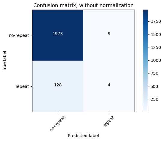
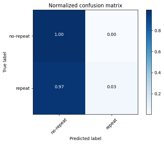
5混淆矩阵 1 2 3 4 5 6 7 8 9 10 11 12 13 14 15 16 17 18 19 20 21 22 23 24 25 26 27 28 29 30 31 32 33 34 35 36 37 38 39 40 41 42 43 44 45 46 47 48 49 50 51 52 53 54 55 56 57 58 59 60 61 62 63 64 65 66 67 68 69 70 import itertoolsimport numpy as npimport matplotlib.pyplot as pltfrom sklearn.model_selection import train_test_splitfrom sklearn.metrics import confusion_matrixfrom sklearn.ensemble import RandomForestClassifier'no-repeat' , 'repeat' ]0 )1 )def plot_confusion_matrix (cm, classes, normalize=False , title='Confusion matrix' , cmap=plt.cm.Blues ):""" This function prints and plots the confusion matrix. Normalization can be applied by setting `normalize=True`. """ if normalize:'float' ) / cm.sum (axis=1 )[:, np.newaxis]print ("Normalized confusion matrix" )else :print ('Confusion matrix, without normalization' )print (cm)'nearest' , cmap=cmap)len (classes))45 )'.2f' if normalize else 'd' max () / 2. for i, j in itertools.product(range (cm.shape[0 ]), range (cm.shape[1 ])):format (cm[i, j], fmt),"center" ,"white" if cm[i, j] > thresh else "black" )'True label' )'Predicted label' )2 ) 'Confusion matrix, without normalization' )True ,'Normalized confusion matrix' )
Confusion matrix, without normalization
[[1973 9]
[ 128 4]]
Normalized confusion matrix
[[1. 0. ]
[0.97 0.03]]
代码解释 函数plot_confusion_matrix解释 :
形参cm是混淆矩阵的数据,classes是分类标签的列表。
normalize参数指示是否应该归一化混淆矩阵。如果设为True,函数则会将每一行的值除以其总和,结果是每一行的数值和为1,这有助于理解每个真实标签的预测分布。title是图表的标题,默认为’Confusion matrix’。cmap=plt.cm.Blues定义了图表使用的颜色映射,默认为蓝色调。
函数内部的步骤包括:
若进行标准化,则对混淆矩阵的每个元素进行规范化,将每一行的值除以该行的总和,并打印“Normalized confusion matrix”(标准化混淆矩阵)。
若不标准化,则打印“Confusion matrix, without normalization”(未标准化的混淆矩阵)。
打印混淆矩阵cm的数值。
使用plt.imshow绘制混淆矩阵的热图,并根据标准化与否设置适当的标题、颜色条卷及颜色映射。
plt.xticks和plt.yticks设置x轴和y轴的刻度标签,旋转x轴标签以便于阅读。使用一个循环在热图上标记每个格子的数值。颜色根据数值与混淆矩阵最大值的一半相比是否较大而决定,以便数值在视觉上更容易区分。
设定x轴和y轴的标签分别为’Predicted label’和’True label’,并调用plt.tight_layout()确保布局正确。
1 2 3 4 5 6 7 8 9 10 11 12 13 14 15 from sklearn.metrics import classification_reportfrom sklearn.ensemble import RandomForestClassifier'no-repeat' , 'repeat' ]0 )1 )print (classification_report(y_test, y_pred, target_names=class_names))
precision recall f1-score support
no-repeat 0.94 1.00 0.97 1982
repeat 0.30 0.02 0.04 132
accuracy 0.94 2114
macro avg 0.62 0.51 0.50 2114
weighted avg 0.90 0.94 0.91 2114
6 不同的分类模型 1 逻辑回归模型 1 2 3 4 5 6 7 8 9 10 11 from sklearn.linear_model import LogisticRegressionfrom sklearn.preprocessing import StandardScaler0 )0 , solver='lbfgs' , multi_class='multinomial' ).fit(X_train, y_train)
0.9380321665089877
代码解释 LogisticRegression(random_state=0, solver='lbfgs', multi_class='multinomial')参数解释
random_state=0:设置随机数种子为0,这样可以在重复运行代码时获得相同的结果。这对于模型的训练和测试是非常有用的。
solver='lbfgs':选择优化算法为L-BFGS。L-BFGS是一种收敛速度较快的优化算法,适用于大规模问题。在这个例子中,我们使用L-BFGS来寻找最优的模型参数。
multi_class='multinomial':设置多分类方式为多类分类器。多类分类器是一种常用的分类方式,它可以处理多类分类问题,例如按钮 clicks、广告点击率预测等。在这个例子中,我们使用多类分类器来预测不同类型的标签。
2.KNN 模型 1 2 3 4 5 6 7 8 9 10 11 from sklearn.neighbors import KNeighborsClassifierfrom sklearn.preprocessing import StandardScaler0 )3 ).fit(X_train, y_train)
0.9252601702932829
3.高斯贝叶斯模型 1 2 3 4 5 6 7 8 9 10 11 from sklearn.naive_bayes import GaussianNBfrom sklearn.preprocessing import StandardScaler0 )
0.3793755912961211
4.决策树模型 1 2 3 4 5 6 7 8 from sklearn import tree0 )
0.8684957426679281
5.Bagging模型 基模型为KNN
1 2 3 4 5 6 7 8 9 from sklearn.ensemble import BaggingClassifierfrom sklearn.neighbors import KNeighborsClassifier0 )0.5 , max_features=0.5 )
0.9375591296121097
6.随机森林模型 1 2 3 4 5 6 7 8 from sklearn.ensemble import RandomForestClassifier0 )10 , max_depth=3 , min_samples_split=12 , random_state=0 )
0.9375591296121097
7.极端随机树模型 1 2 3 4 5 6 7 8 from sklearn.ensemble import ExtraTreesClassifier0 )10 , max_depth=None , min_samples_split=2 , random_state=0 )
0.9309366130558183
229
1 clf.feature_importances_[:10 ]
array([0.08, 0.02, 0.01, 0.02, 0.02, 0.01, 0.01, 0.02, 0.02, 0.01])
8.AdaBoost模型 1 2 3 4 5 6 7 8 from sklearn.ensemble import AdaBoostClassifier0 )10 )
0.9375591296121097
9.GBDT模型 1 2 3 4 5 6 7 8 from sklearn.ensemble import GradientBoostingClassifier0 )10 , learning_rate=1.0 , max_depth=1 , random_state=0 )
0.9375591296121097
10.集成学习 VOTE模型投票
1 2 3 4 5 6 7 8 9 10 11 12 13 14 15 16 17 18 19 20 21 22 from sklearn import datasetsfrom sklearn.model_selection import cross_val_scorefrom sklearn.linear_model import LogisticRegressionfrom sklearn.naive_bayes import GaussianNBfrom sklearn.ensemble import RandomForestClassifierfrom sklearn.ensemble import VotingClassifierfrom sklearn.preprocessing import StandardScaler'lbfgs' , multi_class='multinomial' , random_state=1 )50 , random_state=1 )'lr' , clf1), ('rf' , clf2), ('gnb' , clf3)], voting='hard' )for clf, label in zip ([clf1, clf2, clf3, eclf], ['Logistic Regression' , 'Random Forest' , 'naive Bayes' , 'Ensemble' ]):5 , scoring='accuracy' )print ("Accuracy: %0.2f (+/- %0.2f) [%s]" % (scores.mean(), scores.std(), label))
Accuracy: 0.93 (+/- 0.00) [Logistic Regression]
Accuracy: 0.93 (+/- 0.00) [Random Forest]
Accuracy: 0.39 (+/- 0.02) [naive Bayes]
Accuracy: 0.93 (+/- 0.00) [Ensemble]
11.LGB 模型 1 2 3 4 5 6 7 8 9 10 11 12 13 14 15 16 17 18 19 20 21 22 23 24 25 26 27 28 29 30 31 32 33 34 35 36 37 38 import lightgbm0.4 , random_state=0 )0.5 , random_state=0 )'boosting_type' : 'gbdt' ,'objective' : 'multiclass' ,'metric' : 'multi_logloss' ,'min_child_weight' : 1.5 ,'num_leaves' : 2 **5 ,'lambda_l2' : 10 ,'subsample' : 0.7 ,'colsample_bytree' : 0.7 ,'colsample_bylevel' : 0.7 ,'learning_rate' : 0.03 ,'tree_method' : 'exact' ,'seed' : 2017 ,"num_class" : 2 ,'silent' : True ,10000 100 )]
Early stopping, best iteration is:
[52] valid_0's multi_logloss: 0.237993
1 print ('score : ' , np.mean((pre[:,1 ]>0.5 )==y_valid))
score : 0.937906564163217
12.XGB 模型 1 2 3 4 5 6 7 8 9 10 11 12 13 14 15 16 17 18 19 20 21 22 23 24 25 26 27 28 29 30 31 32 33 34 35 36 37 38 39 import xgboost0.4 , random_state=0 )0.5 , random_state=0 )1 )1 )1 )'booster' : 'gbtree' ,'objective' : 'multi:softprob' ,'eval_metric' : 'mlogloss' ,'gamma' : 1 ,'min_child_weight' : 1.5 ,'max_depth' : 5 ,'lambda' : 100 ,'subsample' : 0.7 ,'colsample_bytree' : 0.7 ,'colsample_bylevel' : 0.7 ,'eta' : 0.03 ,'tree_method' : 'exact' ,'seed' : 2017 ,"num_class" : 2 10000 100 'train' ),'eval' )
[295] train-mlogloss:0.22932 eval-mlogloss:0.23988
[296] train-mlogloss:0.22929 eval-mlogloss:0.23988
[297] train-mlogloss:0.22925 eval-mlogloss:0.23985
[298] train-mlogloss:0.22922 eval-mlogloss:0.23984
[299] train-mlogloss:0.22915 eval-mlogloss:0.23986
[300] train-mlogloss:0.22907 eval-mlogloss:0.23985
1 print ('score : ' , np.mean((pre[:,1 ]>0.3 )==y_valid))
score : 0.937906564163217
7 自己封装模型 7.1 Stacking,Bootstrap,Bagging技术实践 1 2 3 4 5 6 7 8 9 10 """ 导入相关包 """ import pandas as pdimport numpy as npimport lightgbm as lgbfrom sklearn.metrics import f1_scorefrom sklearn.model_selection import train_test_splitfrom sklearn.model_selection import KFoldfrom sklearn.model_selection import StratifiedKFold
1 2 3 4 5 6 7 8 9 10 11 12 13 14 15 16 17 18 19 20 21 22 23 24 25 26 27 28 29 30 31 32 33 34 35 36 37 38 39 40 41 42 43 44 45 46 47 48 49 50 51 52 53 54 55 56 57 58 59 60 61 62 63 64 65 66 67 68 69 70 71 72 73 74 75 76 77 78 79 80 81 82 83 84 85 86 87 88 89 90 91 92 93 94 95 96 97 class SBBTree ():""" SBBTree Stacking,Bootstap,Bagging """ def __init__ ( self, params, stacking_num, bagging_num, bagging_test_size, num_boost_round, callbacks ):""" Initializes the SBBTree. Args: params : lgb params. stacking_num : k_flod stacking. bagging_num : bootstrap num. bagging_test_size : bootstrap sample rate. num_boost_round : boost num. callbacks: callbacks=[lightgbm.early_stopping(stopping_rounds=200) """ self .params = paramsself .stacking_num = stacking_numself .bagging_num = bagging_numself .bagging_test_size = bagging_test_sizeself .num_boost_round = num_boost_roundself .callbacks = callbacksself .model = lgbself .stacking_model = []self .bagging_model = []def fit (self, X, y ):""" fit model. """ if self .stacking_num > 1 :0 ], 2 ))self .SK = StratifiedKFold(n_splits=self .stacking_num, shuffle=True , random_state=1 )for k,(train_index, test_index) in enumerate (self .SK.split(X, y)):self .params,self .num_boost_round,self .callbacksself .stacking_model.append(gbm)1 ] = pred_y1 ].reshape((-1 ,1 )))) else :pass for bn in range (self .bagging_num):self .bagging_test_size, random_state=bn)self .params,10000 ,200 )]self .bagging_model.append(gbm)def predict (self, X_pred ):""" predict test data. """ if self .stacking_num > 1 :0 ], self .stacking_num))for sn,gbm in enumerate (self .stacking_model):1 ).reshape((-1 ,1 )))) else :pass for bn,gbm in enumerate (self .bagging_model):if bn == 0 :else :return pred_out/self .bagging_num
代码解释 这段代码定义了一个名为SBBTree类,表示Stacking, Bootstrap, Bagging这三种集成学习算法的组合。代码中使用了LightGBM框架来训练模型。
详细解释:
类 SBBTree:
__init__ 方法:
类的构造函数用于初始化SBBTree对象,它接受以下参数:
params:LightGBM模型的参数。stacking_num:堆叠的次数,用于k折交叉验证中。bagging_num:Bagging的次数,即bootstrapping的样本集的数量。bagging_test_size:bootstrapping时测试集的比例。num_boost_round:boosting迭代次数。callbacks:回调函数,用于训练过程中提供一些操作,例如早停止。
构造函数内部将传入的参数赋值给类的属性,并初始化了两个列表,stacking_model和bagging_model,分别用于存储来自堆叠的模型和bagging的模型。
fit 方法:
用来训练SBBTree模型。这个方法首先检查如果stacking_num大于1,就会执行k折堆叠,每次迭代都训练一个新的模型并将其添加到stacking_model列表,并且保留预测结果。所有折的预测结果平均后,作为新的特征添加到原有的特征集中。如果stacking_num等于1,预测结果作为新的特征是不被添加的。
接下来的Bagging部分,代码通过train_test_split函数进行多次划分,每一次划分都训练一个新的LightGBM模型,并将每个模型添加到bagging_model列表中。
predict 方法:
用来预测输入的数据X_pred。如果stacking_num大于1,就会使用堆叠过程中得到的模型来对数据进行预测,并将结果平均后作为新特征,再和原始特征进行叠加。然后利用Bagging过程中得到的所有模型对叠加后的特征数据集进行预测。最后,所有Bagging模型的预测结果将求平均值返回最终的预测结果。如果stacking_num等于1,则没有对原始特征叠加新特征的步骤。
该类结合了三种集成算法来提升模型的泛化能力和性能。堆叠(Stacking)是通过将模型的预测结果作为新的特征来训练上层模型;Bootstrap是通过从原数据集中随机抽样来生成新的数据集;Bagging是通过并行地训练多个模型并组合它们的预测结果来减小方差。
这种组合方式通常可以让模型在多样性和稳定性上取得更好的平衡,从而提高预测的准确率。
7.2 测试自己封装的模型类 1 2 3 4 5 6 7 8 9 10 11 12 13 14 15 16 17 18 19 20 21 22 23 24 25 26 27 28 29 30 31 32 33 34 35 36 37 38 39 40 41 42 43 44 45 46 47 48 49 50 51 52 53 54 55 56 57 58 59 60 61 62 63 64 65 66 67 68 69 70 """ TEST CODE """ from sklearn.datasets import make_gaussian_quantilesfrom sklearn import metricsNone , cov=1.0 , n_samples=1000 , n_features=50 , n_classes=2 , shuffle=True , random_state=2 )0.33 , random_state=1 )'task' : 'train' ,'boosting_type' : 'gbdt' ,'objective' : 'binary' ,'metric' : 'auc' ,'num_leaves' : 9 ,'learning_rate' : 0.03 ,'feature_fraction_seed' : 2 ,'feature_fraction' : 0.9 ,'bagging_fraction' : 0.8 ,'bagging_freq' : 5 ,'min_data' : 20 ,'min_hessian' : 1 ,'verbose' : -1 ,'silent' : 0 2 , bagging_num=1 , bagging_test_size=0.33 , num_boost_round=10000 , callbacks=[lightgbm.early_stopping(stopping_rounds=200 )])0 ].reshape((1 ,-1 ))print ('pred' )print (pred)print ('TEST 1 ok' )1 , bagging_num=1 , bagging_test_size=0.33 , num_boost_round=10000 , callbacks=[lightgbm.early_stopping(stopping_rounds=200 )])1 , bagging_num=3 , bagging_test_size=0.33 , num_boost_round=10000 , callbacks=[lightgbm.early_stopping(stopping_rounds=200 )])5 , bagging_num=1 , bagging_test_size=0.33 , num_boost_round=10000 , callbacks=[lightgbm.early_stopping(stopping_rounds=200 )])5 , bagging_num=3 , bagging_test_size=0.33 , num_boost_round=10000 , callbacks=[lightgbm.early_stopping(stopping_rounds=200 )])1 , pred1, pos_label=2 )print ('auc: ' ,metrics.auc(fpr, tpr))1 , pred2, pos_label=2 )print ('auc: ' ,metrics.auc(fpr, tpr))1 , pred3, pos_label=2 )print ('auc: ' ,metrics.auc(fpr, tpr))1 , pred4, pos_label=2 )print ('auc: ' ,metrics.auc(fpr, tpr))
Early stopping, best iteration is:
[26]	valid_0's auc: 0.764161
Training until validation scores don't improve for 200 rounds
Early stopping, best iteration is:
[49]	valid_0's auc: 0.806934
auc:  0.7107286034793483
auc:  0.7791754018169113
auc:  0.7681783074037294
auc:  0.7900989370701387
代码解释 这段测试代码使用了之前定义的SBBTree类,该类是用于构建、训练和预测一个集成学习模型,结合了Stacking、Bootstrap和Bagging策略。
测试代码的步骤包括:
导入make_gaussian_quantiles函数用于生成一个高斯分布的合成数据集,和metrics模块用于评估模型性能。
生成一个含1000个样本、每个样本具有50个特征的数据集,并且标签类别为2。
使用train_test_split把数据集分割成训练集和测试集,测试集大小占33%。
设置LightGBM模型相关的参数params的字典,包括任务类型、梯度提升类型、目标函数、评价指标等。
task:指定当前的任务类型,可以是train(训练)或predict(预测)。boosting_type:指定提升类型,可以是gbdt(梯度提升树)。objective:指定目标函数,可以是binary(二分类)。metric:指定评估指标,可以是auc(Area Under the Curve)。num_leaves:指定叶子节点数。learning_rate:指定学习率。feature_fraction_seed:指定特征fraction的随机种子。feature_fraction:指定特征fraction。bagging_fraction:指定baggingfraction。bagging_freq:指定bagging频率。min_data:指定每个叶子节点上最少的数据样本数。min_hessian:指定每个叶子节点上最小的Hessian值。verbose:指定是否显示日志信息,可以是-1(不显示)或0(显示)。silent:指定是否静默模式,可以是0(不静默)或1(静默)。
进行四个不同设置的测试:
test 1: stacking_num=2, bagging_num=1test 1: stacking_num=1, bagging_num=1test 2: stacking_num=1, bagging_num=3test 3: stacking_num=5, bagging_num=1test 4: stacking_num=5, bagging_num=3
每个测试都实例化了一个SBBTree模型,使用提供的参数进行训练,并对测试集进行预测。
对每个测试的预测结果,使用roc_curve计算真正率(TPR)和假正率(FPR),再使用metrics.auc计算AUC值,并打印出来。y_test+1和pos_label=2的部分是为了使得二元分类的标签与metrics模块的默认正类标签匹配。
这段代码的目标是评估SBBTree不同的堆叠和装袋配置对模型性能(特别是AUC分数)的影响,并打印出模型预测的示例。通过改变堆叠数和装袋数,能看到模型在不同设置下的性能如何变化。
8 天猫复购场景实战 8.1读取特征数据 1 2 3 4 5 6 7 8 9 10 11 12 13 14 15 import pandas as pdimport numpy as npimport lightgbm as lgbfrom sklearn.metrics import f1_scorefrom sklearn.model_selection import train_test_splitfrom sklearn.model_selection import KFoldfrom sklearn.model_selection import StratifiedKFold'./data/train_all.csv' ,nrows=10000 )'./data/test_all.csv' ,nrows=100 )for col in train_data.columns if col not in ['user_id' ,'label' ]]'label' ].values
8.2设置模型参数 1 2 3 4 5 6 7 8 9 10 11 12 13 14 15 16 17 18 19 20 21 22 23 24 params = {'task' : 'train' ,'boosting_type' : 'gbdt' ,'objective' : 'binary' ,'metric' : 'auc' ,'num_leaves' : 9 ,'learning_rate' : 0.03 ,'feature_fraction_seed' : 2 ,'feature_fraction' : 0.9 ,'bagging_fraction' : 0.8 ,'bagging_freq' : 5 ,'min_data' : 20 ,'min_hessian' : 1 ,'verbose' : -1 ,'silent' : 0 5 ,3 ,0.33 ,10000 ,200 )]
8.3模型训练 1 model.fit(train, target)
Training until validation scores don't improve for 200 rounds
Early stopping, best iteration is:
[27]	valid_0's auc: 0.562125
8.4预测结果 1 2 3 4 5 pred = model.predict(test)'user_id' ] = test_data['user_id' ].astype(int )'predict_prob' ] = pred
user_id
predict_prob
0
105600
0.064700
1
110976
0.069873
2
374400
0.069219
3
189312
0.064055
4
189312
0.063837
8.5保存结果 1 2 3 4 5 """ 保留数据头,不保存index """ './data/df_out.csv' ,header=True ,index=False )print ('save OK!' )
save OK!