工业蒸汽预测-05-1模型验证

1 模型评估的概念和方法

1.1 过拟合与欠拟合

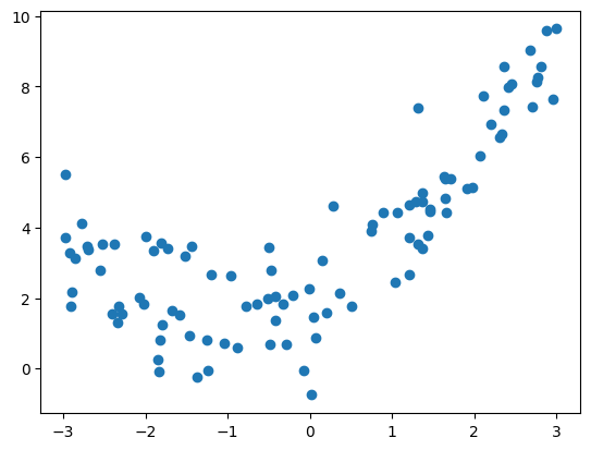
获取并绘制数据集

import numpy as np
import matplotlib.pyplot as plt
%matplotlib inline

np.random.seed(666)
x = np.random.uniform(-3.0, 3.0, size=100)
X = x.reshape(-1, 1)
y = 0.5 * x**2 + x + 2 + np.random.normal(0, 1, size=100)

plt.scatter(x, y)
plt.show()


代码解释

• np.random.seed(666)：设置随机数种子，这样可以确保每次运行代码时生成的随机数是一致的,仅是为了使随机结果可重现，它不直接与散点图有关。。

• x = np.random.uniform(-3.0, 3.0, size=100)：生成一个包含100个在-3.0到3.0之间均匀分布的随机数的一维数组。

• X = x.reshape(-1, 1)：将一维数组 x 转换（重塑reshape）为二维数组 X，其中一列是 x 的值，行数自动计算以匹配原始数据的维度。reshape(-1, 1) 的作用是将一维数组 x 转换为一个二维数组 X，其中 -1 表示自动计算该维度的大小，而 1 表示要创建的数组的列数为1。

• y = 0.5 * x**2 + x + 2 + np.random.normal(0, 1, size=100)：根据给定的二次函数关系生成 y 值，并添加均值为0，标准差为1的正态分布随机噪声。np.random.normal(0, 1, size=100) 是用于生成服从正态分布（高斯分布）的随机数的 NumPy 函数。

  • 0：表示正态分布的均值（mean）为0，即随机数的平均值为0。
  • 1：表示正态分布的标准差（standard deviation）为1，即随机数的离散程度。
  • size=100：表示要生成的随机数的数量为100。

  这个函数将生成一个包含100个元素的一维数组，其中的每个元素都是从均值为0、标准差为1的正态分布中抽取的随机数。在本例中，这些随机数表示了噪声，会被添加到二次曲线的计算结果中，用于在原始数据上引入一些随机性和波动。

  最终，通过 y = 0.5 * x**2 + x + 2 + np.random.normal(0, 1, size=100) 这行代码，我们将按照二次函数关系生成的理想曲线上加入了服从正态分布的随机噪声，得到了最终的观测数据 y。噪声的作用是模拟现实世界中数据的波动性和随机性，使得数据更接近真实情况。

• plt.scatter(x, y)：创建散点图，将 x 和 y 的值传递给 scatter() 函数以绘制数据点。

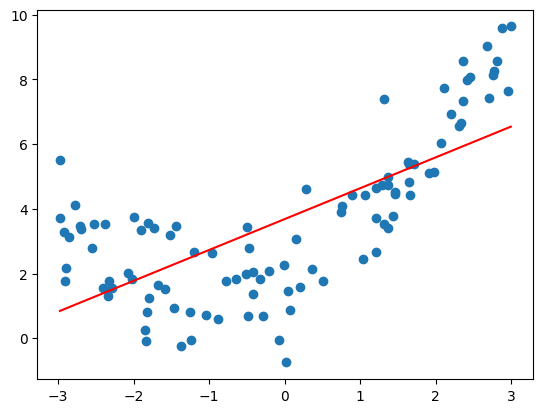
使用线性回归拟合数据

from sklearn.linear_model import LinearRegression

lin_reg = LinearRegression()
lin_reg.fit(X, y)
lin_reg.score(X, y)

0.4953707811865009

准确率为 0.495，比较低，直线拟合数据的程度较低。

使用均方误差判断拟合程度

from sklearn.metrics import mean_squared_error

y_predict = lin_reg.predict(X)
mean_squared_error(y, y_predict)

3.0750025765636577

绘制拟合结果

y_predict = lin_reg.predict(X)
plt.scatter(x, y)
plt.plot(np.sort(x), y_predict[np.argsort(x)], color='r')
plt.show()

​
​

代码解释

plt.plot(np.sort(x), y_predict[np.argsort(x)], color='r') 用于在图形中绘制拟合直线。

• np.sort(x)：将输入特征 x 进行升序排序，得到排序后的数组。这是因为 x 的顺序可能是乱序的，绘制拟合直线时需要按照从小到大的顺序连接数据点。

• y_predict[np.argsort(x)]：根据 x 的排序结果，对预测值 y_predict 进行重新排列。np.argsort(x) 返回的是 x 的索引按照升序排列的结果。通过使用这个索引数组对 y_predict 进行切片操作，可以按照相同的顺序重新排列预测值，使其与排序后的 x 相对应。

• color='r'：指定拟合直线的颜色为红色 (‘r’)。

将排序后的输入特征 x 与重新排列的预测值 y_predict 作为参数传递给 plot() 函数，绘制拟合直线。通过按照从小到大的顺序连接数据点，可以在图形中展示出线性回归模型对原始数据的拟合程度。

使用多项式回归拟合

• 首先封装Pipeline管道，这样便于下一步灵活调整多项式回归模型参数

from sklearn.pipeline import Pipeline 
from sklearn.preprocessing import PolynomialFeatures
from sklearn.preprocessing import StandardScaler

def PolynomialRegression(degree):
    return Pipeline([
        ('poly', PolynomialFeatures(degree=degree)),
        ('std_scaler', StandardScaler()),
        ('lin_reg', LinearRegression())
    ])

代码解释

用于创建多项式回归模型的函数。使用sklearn库中的Pipeline类来构建一个机器学习工作流程，包括多项式特征转换、标准化和线性回归模型。

• from sklearn.pipeline import Pipeline: Pipeline类，用于将多个数据处理步骤和机器学习模型封装在一起，形成一个流水线。

• from sklearn.preprocessing import PolynomialFeatures: PolynomialFeatures类，用于进行多项式特征转换。

• from sklearn.preprocessing import StandardScaler: StandardScaler类，用于进行特征标准化（特征缩放）。

• def PolynomialRegression(degree): 定义PolynomialRegression函数，接受参数degree，表示多项式的次数。

• return Pipeline([...]): 使用Pipeline类创建一个机器学习工作流程并返回。Pipeline类接受一个由元组构成的列表作为参数，每个元组代表工作流程中的一个步骤。

  • ('poly', PolynomialFeatures(degree=degree)): 多项式特征转换步骤，将输入特征转换为指定次数的多项式特征。使用PolynomialFeatures类，并将其实例命名为’poly’。

  • ('std_scaler', StandardScaler()): 标准化步骤，对多项式特征进行特征缩放，使特征的均值为0，标准差为1。使用StandardScaler类，并将其实例命名为’std_scaler’。

  • ('lin_reg', LinearRegression()): 线性回归模型步骤，用于拟合多项式特征和目标变量之间的关系。使用LinearRegression类，并将其实例命名为’lin_reg’。

创建一个多项式回归模型，通过使用多项式特征转换和标准化来提高模型的性能。可以根据需要选择不同的多项式次数，从而得到不同复杂度的模型。

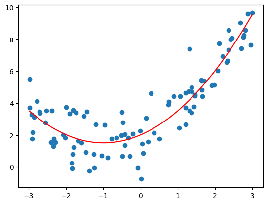
• 使用 Pipeline 拟合数据：degree = 2

poly2_reg = PolynomialRegression(degree=2)
poly2_reg.fit(X, y)

y2_predict = poly2_reg.predict(X)

# 比较真值和预测值的均方误差
mean_squared_error(y, y2_predict)

1.0987392142417858

• 绘制拟合结果

plt.scatter(x, y)
plt.plot(np.sort(x), y2_predict[np.argsort(x)], color='r')
plt.show()

​
​

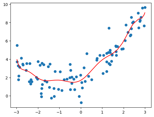
• 调整 degree = 10

poly10_reg = PolynomialRegression(degree=10)
poly10_reg.fit(X, y)

y10_predict = poly10_reg.predict(X)
print(mean_squared_error(y, y10_predict))


plt.scatter(x, y)
plt.plot(np.sort(x), y10_predict[np.argsort(x)], color='r')
plt.show()

1.0508466763764126


• 调整 degree = 100

poly100_reg = PolynomialRegression(degree=100)
poly100_reg.fit(X, y)

y100_predict = poly100_reg.predict(X)
print(mean_squared_error(y, y100_predict))


plt.scatter(x, y)
plt.plot(np.sort(x), y100_predict[np.argsort(x)], color='r')
plt.show()

0.6807802342342404


• 分析
  1. degree=2：均方误差为 1.0987392142417858；
  2. degree=10：均方误差为 1.0508466763764126；
  3. degree=100：均方误差为 0.6807802342342404；
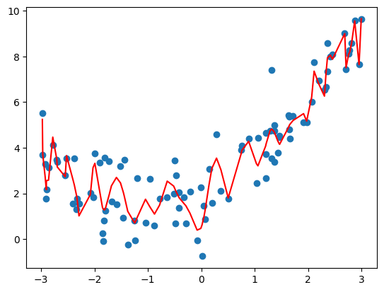
  4. degree 越大拟合的效果越好，因为样本点是一定的，我们总能找到一条曲线将所有的样本点拟合，也就是说将所有的样本点都完全落在这根曲线上，使得整体的均方误差为 0；
  5. 红色曲线并不是所计算出的拟合曲线，而此红色曲线只是原有的数据点对应的 y 的预测值连接出来的结果，而且有的地方没有数据点，因此连接的结果和原来的曲线不一样；

1.2 交叉验证

1.2.1交叉验证迭代器

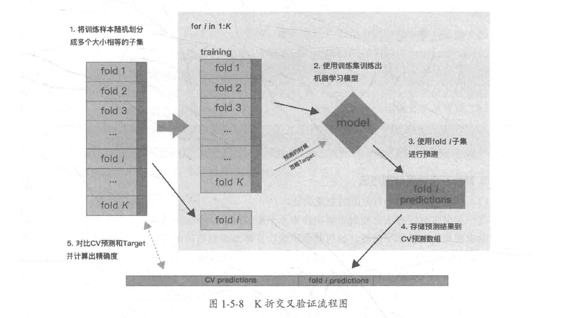
K折交叉验证：K-Fold Cross Validation,是将原始数据分成K组（一般是均分）,称为折叠 (fold)，然后将每个子集数据分别做一次验证集，其余的K-1组子集数据作为训练集，这样就会得到K个模型，将K个模型最终的验证集的分类准确率取平均值，作为K折交叉验证分类器的性能指标。通常设置K大于或等于3。


K折重复多次： RepeatedKFold 重复 K-Fold n 次。当需要运行时可以使用它 KFold n 次，在每次重复中产生不同的分割。

留一交叉验证： LeaveOneOut (或 LOO) 是一个简单的交叉验证。每个训练集都由除了一个样本以外的其余所有样本组成的，留下的一个样本组成检验集。 这样，对于 n 个样本，我们有 n 个不同的训练集和 n 个不同的测试集。因此LOO-CV会得到N个模型，用N个模型最终的验证集的分类准确率的平均数作为分类器的性能指标。这种交叉验证程序不会浪费太多数据，因为只有一个样本是从训练集中删除掉的。


留P交叉验证： LeavePOut 与 LeaveOneOut 非常相似，因为它通过从整个集合中删除 p 个样本来创建所有可能的训练/测试集。对于 n 个样本，这产生了 (n,p) 个 训练-测试对。与 LeaveOneOut 和 KFold 不同，当 p > 1 时，测试集会重叠。

用户自定义数据集划分： ShuffleSplit 迭代器将会生成一个用户给定数量的独立的训练/测试数据划分。样例首先被打散然后划分为一对训练测试集合。

设置每次生成的随机数相同： 可以通过设定明确的 random_state ，使得伪随机生成器的结果可以重复。

1.2.2基于类标签、具有分层的交叉验证迭代器

如何解决样本不平衡问题？ 使用StratifiedKFold和StratifiedShuffleSplit 分层抽样。 一些分类问题在目标类别的分布上可能表现出很大的不平衡性：例如，可能会出现比正样本多数倍的负样本。在这种情况下，建议采用如 StratifiedKFold 和 StratifiedShuffleSplit 中实现的分层抽样方法，确保相应的类别频率在每个训练和验证的折叠中大致得以保留。

StratifiedKFold是 k-fold 的变种，会返回 stratified（分层） 的折叠：每个小集合中，各个类别的样例比例大致和完整数据集中相同。

StratifiedShuffleSplit是 ShuffleSplit 的一个变种，会返回直接的划分，比如：创建一个划分，但是划分中每个类的比例和完整数据集中的相同。

1.2.3用于分组数据的交叉验证迭代器

如何进一步测试模型的泛化能力？ 留出一组特定的不属于测试集和训练集的数据。有时我们想知道在一组特定的 groups 上训练的模型是否能很好地适用于看不见的新数据。为了衡量这一点，我们需要确保验证对象中的所有样本均未在配对训练折叠中出现过，采用的办法就是留出一组特定的不属于测试集和训练集的数据，常用的方法包括GroupKFold,LeaveOneGroupOut,LeavePGroupsOut,GroupShuffleSplit.

GroupKFold是 k-fold 的变体，它确保同一个 group 在测试和训练集中都不被表示。 例如，如果数据是从不同的组获得的，每个组又有多个样本，并且如果模型足够灵活，能高度从指定的特征中学习，则可能存在很好地拟合训练的组，但不能很好地预测不存在于训练组中的样本，GroupKFold 可以检测到这种过拟合的情况。

LeaveOneGroupOut是一个交叉验证方案，它根据用户提供的 array of integer groups （整数组的数组）来区别不同的组，以此来提供样本。这个组信息可以用来编码任意域特定的预定义交叉验证折叠。每个训练集都是由除特定组别以外的所有样本构成的。

LeavePGroupsOut类似于 LeaveOneGroupOut ，但为每个训练/测试集删除与 P 组有关的样本。

GroupShuffleSplit迭代器是 ShuffleSplit 和 LeavePGroupsOut 的组合，它生成一个随机划分分区的序列，其中为每个分组提供了一个组子集。

1.2.4 时间序列分割

TimeSeriesSplit 也是K-Fold的一个变种，首先返回K折作为训练数据集，把K+1折作为测试数据集。请注意，与标准的交叉验证方法不同，有关时间序列的样本切分必须保证时间上的顺序性，不能用未来的数据去验证现在数据的正确性，只能使用时间上之前一段的数据建模，而用后一段时间的数据来验证模型预测的效果，这也是时间序列数据在做模型验证划分数据时与其他常规数据切分的区别。

from sklearn.model_selection import train_test_split,cross_val_score,cross_validate # 交叉验证所需的函数
from sklearn.model_selection import KFold,LeaveOneOut,LeavePOut,ShuffleSplit # 交叉验证所需的子集划分方法
from sklearn.model_selection import StratifiedKFold,StratifiedShuffleSplit # 分层分割
from sklearn.model_selection import GroupKFold,LeaveOneGroupOut,LeavePGroupsOut,GroupShuffleSplit # 分组分割
from sklearn.model_selection import TimeSeriesSplit # 时间序列分割
from sklearn import datasets  # 自带数据集
from sklearn import svm  # SVM算法
from sklearn import preprocessing  # 预处理模块
from sklearn.metrics import recall_score  # 模型度量

iris = datasets.load_iris()  # 加载数据集
print('样本集大小：',iris.data.shape,iris.target.shape)

# ===================================数据集划分,训练模型==========================
X_train, X_test, y_train, y_test = train_test_split(iris.data, iris.target, test_size=0.4, random_state=0)  # 交叉验证划分训练集和测试集.test_size为测试集所占的比例
print('训练集大小：',X_train.shape,y_train.shape)  # 训练集样本大小
print('测试集大小：',X_test.shape,y_test.shape)  # 测试集样本大小
clf = svm.SVC(kernel='linear', C=1).fit(X_train, y_train) # 使用训练集训练模型
print('准确率：',clf.score(X_test, y_test))  # 计算测试集的度量值（准确率）


#  如果涉及到归一化，则在测试集上也要使用训练集模型提取的归一化函数。
scaler = preprocessing.StandardScaler().fit(X_train)  # 通过训练集获得归一化函数模型。（也就是先减几，再除以几的函数）。在训练集和测试集上都使用这个归一化函数
X_train_transformed = scaler.transform(X_train)
clf = svm.SVC(kernel='linear', C=1).fit(X_train_transformed, y_train) # 使用训练集训练模型
X_test_transformed = scaler.transform(X_test)
print(clf.score(X_test_transformed, y_test))  # 计算测试集的度量值（准确度）

# ===================================直接调用交叉验证评估模型==========================
clf = svm.SVC(kernel='linear', C=1)
scores = cross_val_score(clf, iris.data, iris.target, cv=5)  #cv为迭代次数。
print(scores)  # 打印输出每次迭代的度量值（准确度）
print("Accuracy: %0.2f (+/- %0.2f)" % (scores.mean(), scores.std() * 2))  # 获取置信区间。（也就是均值和方差）

# ===================================多种度量结果======================================
scoring = ['precision_macro', 'recall_macro'] # precision_macro为精度（准确率），recall_macro为召回率
scores = cross_validate(clf, iris.data, iris.target, scoring=scoring,cv=5, return_train_score=True)
sorted(scores.keys())
print('测试结果：',scores)  # scores类型为字典。包含训练得分，拟合次数， score-times （得分次数）


# ==================================K折交叉验证、留一交叉验证、留p交叉验证、随机排列交叉验证==========================================
# k折划分子集
kf = KFold(n_splits=2)
for train, test in kf.split(iris.data):
    print("k折划分：%s %s" % (train.shape, test.shape))
    break

# 留一划分子集
loo = LeaveOneOut()
for train, test in loo.split(iris.data):
    print("留一划分：%s %s" % (train.shape, test.shape))
    break

# 留p划分子集
lpo = LeavePOut(p=2)
for train, test in loo.split(iris.data):
    print("留p划分：%s %s" % (train.shape, test.shape))
    break

# 随机排列划分子集
ss = ShuffleSplit(n_splits=3, test_size=0.25,random_state=0)
for train_index, test_index in ss.split(iris.data):
    print("随机排列划分：%s %s" % (train.shape, test.shape))
    break

# ==================================分层K折交叉验证、分层随机交叉验证==========================================
skf = StratifiedKFold(n_splits=3)  #各个类别的比例大致和完整数据集中相同
for train, test in skf.split(iris.data, iris.target):
    print("分层K折划分：%s %s" % (train.shape, test.shape))
    break

skf = StratifiedShuffleSplit(n_splits=3)  # 划分中每个类的比例和完整数据集中的相同
for train, test in skf.split(iris.data, iris.target):
    print("分层随机划分：%s %s" % (train.shape, test.shape))
    break


# ==================================组 k-fold交叉验证、留一组交叉验证、留 P 组交叉验证、Group Shuffle Split==========================================
X = [0.1, 0.2, 2.2, 2.4, 2.3, 4.55, 5.8, 8.8, 9, 10]
y = ["a", "b", "b", "b", "c", "c", "c", "d", "d", "d"]
groups = [1, 1, 1, 2, 2, 2, 3, 3, 3, 3]

# k折分组
gkf = GroupKFold(n_splits=3)  # 训练集和测试集属于不同的组
for train, test in gkf.split(X, y, groups=groups):
    print("组 k-fold分割：%s %s" % (train, test))

# 留一分组
logo = LeaveOneGroupOut()
for train, test in logo.split(X, y, groups=groups):
    print("留一组分割：%s %s" % (train, test))

# 留p分组
lpgo = LeavePGroupsOut(n_groups=2)
for train, test in lpgo.split(X, y, groups=groups):
    print("留 P 组分割：%s %s" % (train, test))

# 随机分组
gss = GroupShuffleSplit(n_splits=4, test_size=0.5, random_state=0)
for train, test in gss.split(X, y, groups=groups):
    print("随机分割：%s %s" % (train, test))


# ==================================时间序列分割==========================================
tscv = TimeSeriesSplit(n_splits=3)
TimeSeriesSplit(max_train_size=None, n_splits=3)
for train, test in tscv.split(iris.data):
    print("时间序列分割：%s %s" % (train, test))

样本集大小： (150, 4) (150,)
训练集大小： (90, 4) (90,)
测试集大小： (60, 4) (60,)
准确率： 0.9666666666666667
0.9333333333333333
[0.96666667 1.         0.96666667 0.96666667 1.        ]
Accuracy: 0.98 (+/- 0.03)
测试结果： {'fit_time': array([0.00000000e+00, 1.00016594e-03, 1.00016594e-03, 4.05311584e-05,
       0.00000000e+00]), 'score_time': array([0.00100017, 0.        , 0.00100017, 0.        , 0.        ]), 'test_precision_macro': array([0.96969697, 1.        , 0.96969697, 0.96969697, 1.        ]), 'train_precision_macro': array([0.97674419, 0.97674419, 0.99186992, 0.98412698, 0.98333333]), 'test_recall_macro': array([0.96666667, 1.        , 0.96666667, 0.96666667, 1.        ]), 'train_recall_macro': array([0.975     , 0.975     , 0.99166667, 0.98333333, 0.98333333])}
k折划分：(75,) (75,)
留一划分：(149,) (1,)
留p划分：(149,) (1,)
随机排列划分：(149,) (1,)
分层K折划分：(100,) (50,)
分层随机划分：(135,) (15,)
组 k-fold分割：[0 1 2 3 4 5] [6 7 8 9]
组 k-fold分割：[0 1 2 6 7 8 9] [3 4 5]
组 k-fold分割：[3 4 5 6 7 8 9] [0 1 2]
留一组分割：[3 4 5 6 7 8 9] [0 1 2]
留一组分割：[0 1 2 6 7 8 9] [3 4 5]
留一组分割：[0 1 2 3 4 5] [6 7 8 9]
留 P 组分割：[6 7 8 9] [0 1 2 3 4 5]
留 P 组分割：[3 4 5] [0 1 2 6 7 8 9]
留 P 组分割：[0 1 2] [3 4 5 6 7 8 9]
随机分割：[0 1 2] [3 4 5 6 7 8 9]
随机分割：[3 4 5] [0 1 2 6 7 8 9]
随机分割：[3 4 5] [0 1 2 6 7 8 9]
随机分割：[3 4 5] [0 1 2 6 7 8 9]
时间序列分割：[ 0  1  2  3  4  5  6  7  8  9 10 11 12 13 14 15 16 17 18 19 20 21 22 23
 24 25 26 27 28 29 30 31 32 33 34 35 36 37 38] [39 40 41 42 43 44 45 46 47 48 49 50 51 52 53 54 55 56 57 58 59 60 61 62
 63 64 65 66 67 68 69 70 71 72 73 74 75]
时间序列分割：[ 0  1  2  3  4  5  6  7  8  9 10 11 12 13 14 15 16 17 18 19 20 21 22 23
 24 25 26 27 28 29 30 31 32 33 34 35 36 37 38 39 40 41 42 43 44 45 46 47
 48 49 50 51 52 53 54 55 56 57 58 59 60 61 62 63 64 65 66 67 68 69 70 71
 72 73 74 75] [ 76  77  78  79  80  81  82  83  84  85  86  87  88  89  90  91  92  93
  94  95  96  97  98  99 100 101 102 103 104 105 106 107 108 109 110 111
 112]
时间序列分割：[  0   1   2   3   4   5   6   7   8   9  10  11  12  13  14  15  16  17
  18  19  20  21  22  23  24  25  26  27  28  29  30  31  32  33  34  35
  36  37  38  39  40  41  42  43  44  45  46  47  48  49  50  51  52  53
  54  55  56  57  58  59  60  61  62  63  64  65  66  67  68  69  70  71
  72  73  74  75  76  77  78  79  80  81  82  83  84  85  86  87  88  89
  90  91  92  93  94  95  96  97  98  99 100 101 102 103 104 105 106 107
 108 109 110 111 112] [113 114 115 116 117 118 119 120 121 122 123 124 125 126 127 128 129 130
 131 132 133 134 135 136 137 138 139 140 141 142 143 144 145 146 147 148
 149]

2 模型调参

参数可分为两类：过程影响类参数和子模型影响类参数。

2.1 网格搜索

Grid Search：一种穷举搜索的调参手段；穷举搜索：在所有候选的参数选择中，通过循环遍历，尝试每一种可能性，表现最好的参数就是最终的结果。

简单的网格搜索

from sklearn.datasets import load_iris
from sklearn.svm import SVC
from sklearn.model_selection import train_test_split

iris = load_iris()

X_train,X_test,y_train,y_test = train_test_split(iris.data,iris.target,random_state=0)
print("Size of training set:{} size of testing set:{}".format(X_train.shape[0],X_test.shape[0]))

####   grid search start
best_score = 0
for gamma in [0.001,0.01,0.1,1,10,100]:
    for C in [0.001,0.01,0.1,1,10,100]:
        svm = SVC(gamma=gamma,C=C)#对于每种参数可能的组合，进行一次训练；
        svm.fit(X_train,y_train)
        score = svm.score(X_test,y_test)
        if score > best_score:#找到表现最好的参数
            best_score = score
            best_parameters = {'gamma':gamma,'C':C}
####   grid search end

print("Best score:{:.2f}".format(best_score))
print("Best parameters:{}".format(best_parameters))

Size of training set:112 size of testing set:38
Best score:0.97
Best parameters:{'gamma': 0.001, 'C': 100}

2.2 学习曲线和验证曲线

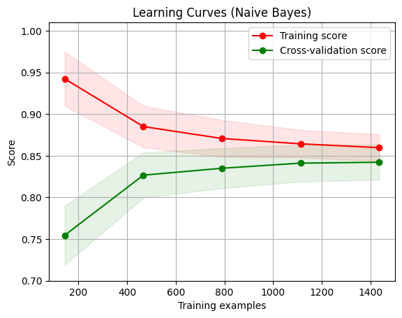
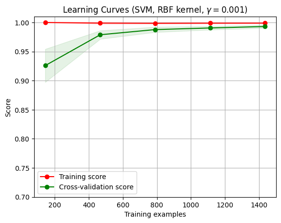
2.2.1 学习曲线

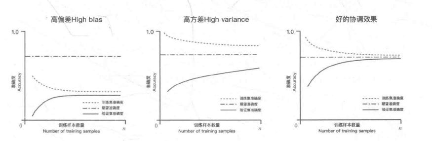
通过学习曲线来绘制模型在训练集和交叉验证集上的准确率，观察模型在新数据上的表现进而判断模型的方差或偏差是否过高，以及增大训练集是否可以减小过拟合。

import numpy as np
import matplotlib.pyplot as plt

from sklearn.naive_bayes import GaussianNB # 高斯朴素贝叶斯分类器
from sklearn.svm import SVC # 支持向量机（SVM）分类器

from sklearn.datasets import load_digits # 手写数字数据集
from sklearn.model_selection import learning_curve # 绘制学习曲线
from sklearn.model_selection import ShuffleSplit # 创建随机交叉验证策略

# 绘制学习曲线
def plot_learning_curve(estimator, title, X, y, ylim=None, cv=None,
                        n_jobs=1, train_sizes=np.linspace(.1, 1.0, 5)):
    plt.figure()
    plt.title(title)
    if ylim is not None:
        plt.ylim(*ylim)
    plt.xlabel("Training examples")
    plt.ylabel("Score")
    train_sizes, train_scores, test_scores = learning_curve(
        estimator, X, y, cv=cv, n_jobs=n_jobs, train_sizes=train_sizes)
    train_scores_mean = np.mean(train_scores, axis=1)
    train_scores_std = np.std(train_scores, axis=1)
    test_scores_mean = np.mean(test_scores, axis=1)
    test_scores_std = np.std(test_scores, axis=1)
    plt.grid() # 在绘图中添加网格线

    plt.fill_between(train_sizes, train_scores_mean - train_scores_std,
                     train_scores_mean + train_scores_std, alpha=0.1,
                     color="r")
    plt.fill_between(train_sizes, test_scores_mean - test_scores_std,
                     test_scores_mean + test_scores_std, alpha=0.1, color="g")
    plt.plot(train_sizes, train_scores_mean, 'o-', color="r",
             label="Training score")
    plt.plot(train_sizes, test_scores_mean, 'o-', color="g",
             label="Cross-validation score")

    plt.legend(loc="best")
    return plt 

代码解释

定义 plot_learning_curve 的函数。该函数用于绘制学习曲线，评估模型在不同训练集大小下的性能表现。

参数说明：

• estimator：要评估的分类器或回归器对象
• title：图形的标题
• X：特征矩阵
• y：目标变量
• ylim：y轴上的取值范围
• cv：交叉验证策略对象，默认为None
• n_jobs：并行处理的工作进程数，默认为1
• train_sizes：可选的训练集大小，用于绘制学习曲线，默认为 [0.1, 0.3, 0.5, 0.7, 0.9, 1.0]

函数内部的操作如下：

1. 创建一个新的图形对象
2. 设置图形的标题和轴标签
3. 如果指定了 ylim 参数，则设置 y 轴上的取值范围
4. 调用 learning_curve 方法计算训练集和测试集的得分 (train_scores 和 test_scores)，以及相应的均值 (train_scores_mean 和 test_scores_mean) 和标准差 (train_scores_std 和 test_scores_std)
5. 绘制学习曲线图形：使用 fill_between 方法绘制训练集和测试集得分的区间范围，使用 plot 方法绘制训练集和测试集得分的均值
6. 添加图例并显示网格线
7. 返回图形对象

部分代码详解：

1. plt.ylim(*ylim)
   • plt.ylim 是 Matplotlib 库中的一个函数，用于设置 y 轴上的取值范围。该函数接受两个参数，表示 y 轴的下限和上限。在上述代码中，plt.ylim(*ylim) 表示将传入的 ylim 参数解包，并将解包后得到的两个值分别作为下限和上限传递给 plt.ylim 函数。
   • *ylim 使用了 * 运算符，表示将 ylim 参数解包。当函数调用时，如果一个参数前面有 *，则表示将该参数解包为多个独立的值。在这里，*ylim 的作用是将 ylim 参数解包为两个值，以便传递给 plt.ylim 函数。解包后的第一个值将成为下限，第二个值将成为上限。

---

2. learning_curve 函数

from sklearn.model_selection import learning_curve

train_sizes, train_scores, test_scores = learning_curve(
    estimator, X, y, train_sizes=None, cv=None, scoring=None, n_jobs=None, 
    shuffle=True, random_state=None, verbose=0, error_score='raise', **kwargs)

参数说明： 

• estimator: 所使用的分类或回归算法。
• X: 特征矩阵。
• y: 目标变量。
• train_sizes: 是否自定义训练集大小，如果指定为 None，则默认生成 5 个等间隔的训练集大小，最小大小为 0.1，最大大小为 1，即 train_sizes=np.linspace(0.1, 1.0, 5)。
• cv: 交叉验证策略对象，默认为 None。可以使用整数、用于指定折叠数量的交叉验证生成器，或者用于划分数据集的可迭代对象。
• scoring: 模型性能评估指标，可以选择预定义的性能评估指标字符串，或者自定义的评估函数。
• n_jobs: 并行处理的工作进程数，默认为 None，表示使用单个进程（如果设为 -1，则使用所有可用的CPU）。
• shuffle: 每次交叉验证时，是否对训练数据顺序进行随机洗牌。
• random_state: 用于生成随机数的种子，设定后可以保证每次运行都能得到相同的结果。
• verbose: 控制输出信息的详细程度。
• error_score: 如果某个参数设置导致模型无法有效的训练，则会产生一个错误分数。

函数返回三个数组：

• train_sizes: 训练集大小的数组。
• train_scores: 每组训练集大小下模型在训练集上的得分的数组。
• test_scores: 每组训练集大小下模型在测试集上的得分的数组。

---

3. plt.fill_between() 函数

用于在两条曲线之间填充颜色或填充区域。它可以用于可视化误差范围、置信区间或数据集分布等情况。文中即在学习曲线图中填充了训练集得分均值的上下方差区域。具体来说，它将训练集得分均值减去标准差的结果和加上标准差的结果之间的区域进行填充，并指定了填充的颜色。

plt.fill_between(x, y1, y2=0, where=None, interpolate=False, step=None, **kwargs)

参数说明：

• x：表示 x 轴上的数据点。
• y1：表示第一条曲线的 y 值。
• y2：表示第二条曲线的 y 值，默认为 0。如果设置为数组，则必须和 y1 的长度相同，用于填充两条曲线之间的区域。
• where：一个条件数组或布尔表达式，指定应该填充区域的位置。默认为 None，表示在整个 x 范围内填充区域。
• interpolate：一个布尔值，指定是否对填充区域进行插值。默认为 False，表示不进行插值。
• step：一个字符串，指定填充区域的类型，可以是 “pre”、”post” 或者 “mid”。默认为 None，表示不进行任何变化。
• **kwargs：可选参数，用于指定填充区域的属性，例如填充颜色、透明度等。

常用属性参数：

• color：指定填充的颜色。
• alpha：指定填充颜色的透明度。
• edgecolor：指定边缘线的颜色。
• linewidth：指定边缘线的宽度。

---

4. plt.plot() 函数
   用于绘制线图。可以用来可视化数据集、绘制函数曲线等。

plt.plot(x, y, fmt, **kwargs)

参数说明：

• x：表示 x 轴上的数据点。
• y：表示 y 轴上的数据点。
• fmt：一个可选参数，用于指定线条的样式，包括颜色、线型和标记。例如，’b-‘ 表示蓝色实线；’g–’ 表示绿色虚线；’ro’ 表示红色圆点。参考下面的属性参数部分。
• **kwargs：可选参数，用于设置线条的其他属性，例如线宽、标签、透明度等。

常用的属性参数：

• color：指定线条的颜色，例如 ‘red’、’green’。
• linestyle：指定线条的样式，例如 ‘-‘（实线）、’–’（虚线）。
• marker：指定标记类型，例如 ‘o’（圆点）、’s’（方块）。
• linewidth：指定线条的宽度。
• label：指定线条的标签。

digits = load_digits()
X, y = digits.data, digits.target


title = "Learning Curves (Naive Bayes)"
# Cross validation with 100 iterations to get smoother mean test and train
# score curves, each time with 20% data randomly selected as a validation set.
cv = ShuffleSplit(n_splits=100, test_size=0.2, random_state=0)

estimator = GaussianNB()
plot_learning_curve(estimator, title, X, y, ylim=(0.7, 1.01), cv=cv, n_jobs=1)

<module 'matplotlib.pyplot' from 'D:\\Development\\anaconda3\\envs\\ml\\lib\\site-packages\\matplotlib\\pyplot.py'>

​
​

代码解释

ShuffleSplit()
用于生成随机划分的训练集和测试集。它在每次划分时都会对数据集进行洗牌（随机打乱），以确保训练集和测试集的划分是随机的。

两个主要作用：

1. 评估模型性能：通过多次随机划分数据集并在每个划分上训练和评估模型，可以得到模型在不同训练集和测试集上的性能指标，如准确率、回归的 R2 分数等。
2. 参数调优：通过交叉验证评估模型的性能，可以帮助选择最优的模型参数。例如，在网格搜索调优中使用 ShuffleSplit() 可以评估不同参数组合下的模型性能。

常用参数：

• n_splits：指定将数据集划分为多少个不同的训练集和测试集的组合。
• test_size：指定测试集的大小。可以是一个整数（表示样本数量），也可以是一个浮点数（表示比例）。
• train_size：指定训练集的大小。可以是一个整数（表示样本数量），也可以是一个浮点数（表示比例）。与 test_size 二选一。
• random_state：指定随机种子。保持相同的 random_state 值会得到相同的随机结果。

title = "Learning Curves (SVM, RBF kernel, $\gamma=0.001$)"
# SVC is more expensive so we do a lower number of CV iterations:
cv = ShuffleSplit(n_splits=10, test_size=0.2, random_state=0)
estimator = SVC(gamma=0.001)
plot_learning_curve(estimator, title, X, y, (0.7, 1.01), cv=cv, n_jobs=1)

<module 'matplotlib.pyplot' from 'D:\\Development\\anaconda3\\envs\\ml\\lib\\site-packages\\matplotlib\\pyplot.py'>

​
​

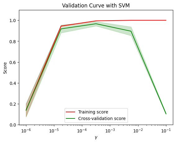
2.2.2 验证曲线

import matplotlib.pyplot as plt
import numpy as np
from sklearn.datasets import load_digits
from sklearn.svm import SVC
from sklearn. model_selection import validation_curve

digits = load_digits()
X, y = digits.data, digits.target

param_range = np.logspace(-6, -1, 5)
train_scores, test_scores = validation_curve(
    SVC(), X, y, param_name="gamma", param_range=param_range,
    cv=10, scoring="accuracy", n_jobs=1)
train_scores_mean = np.mean(train_scores, axis=1)
train_scores_std = np.std(train_scores, axis=1)
test_scores_mean = np.mean(test_scores, axis=1)
test_scores_std = np.std(test_scores, axis=1)

plt.title("Validation Curve with SVM")
plt.xlabel("$\gamma$")
plt.ylabel("Score")
plt.ylim(0.0, 1.1)
plt.semilogx(param_range, train_scores_mean, label="Training score", color="r")
plt.fill_between(param_range, train_scores_mean - train_scores_std,
                 train_scores_mean + train_scores_std, alpha=0.2, color="r")
plt.semilogx(param_range, test_scores_mean, label="Cross-validation score",
             color="g")
plt.fill_between(param_range, test_scores_mean - test_scores_std,
                 test_scores_mean + test_scores_std, alpha=0.2, color="g")
plt.legend(loc="best")
plt.show()

​
​

代码解释

1. np.logspace()
   用于生成在对数刻度上均匀分布的数值序列。

np.logspace(start, stop, num=50, endpoint=True, base=10.0, dtype=None)

参数解释：

• start：起始值，表示数列的起点。
• stop：结束值，表示数列的终点。
• num：要生成的数的个数，默认为 50。
• endpoint：是否包含终点值，默认为 True。如果为 False，则生成的数列不包含结束值。
• base：对数的底数，默认为 10.0。
• dtype：返回值的数据类型。

np.logspace() 函数将起始值和结束值在对数刻度上等分为指定个数的数列，并返回该数列。

param_range = np.logspace(-6, -1, 5) 生成一个从 10 的 -6 次方到 10 的 -1 次方之间的等比数列，共包含 5 个值。

---

2. validation_curve()函数
   用于绘制验证曲线（validation curve）。

sklearn.model_selection.validation_curve(estimator, X, y, param_name, param_range, cv=None, scoring=None, n_jobs=None, pre_dispatch="all", verbose=0)

参数解释：

• estimator：用于训练和预测的模型对象。
• X：特征数据。
• y：目标数据。
• param_name：要调整的控制模型行为的参数名称。
• param_range：参数的取值范围。
• cv：交叉验证的折数，默认为 None。如果为整数，则表示 K 折交叉验证；如果为交叉验证生成器对象，则可以更灵活地定义交叉验证策略。
• scoring：评估指标，默认为 None。如果为 None，则使用模型的默认评估指标；如果为字符串或可调用对象，则使用指定的评估指标。
• n_jobs：并行运行的作业数，默认为 None，表示使用单个进程运行。
• pre_dispatch：控制并行运行的内部作业数量，默认为 “all”，表示并行运行所有作业。
• verbose：详细程度，默认为 0，表示不输出执行信息；大于 0 的值表示输出一些执行信息。

validation_curve() 函数通过在给定参数的不同取值上计算训练得分和验证得分，绘制了模型复杂度（参数）与性能之间的关系曲线。它有助于判断模型在不同参数取值下的过/欠拟合情况，并选择最佳参数取值。

返回值：

• 返回一个包含训练得分和验证得分的元组 (train_scores, test_scores)。每个得分都是一个二维数组，行数表示不同参数取值，列数表示交叉验证的次数。

本示例中，我们使用 SVM 模型对 iris 数据集进行训练。param_name="gamma" 表示将调整 gamma 参数的值。param_range 定义了 gamma 参数的取值范围。

cv=5 表示进行 5 折交叉验证。scoring="accuracy" 表示评估指标为准确率。

---

3. plt.semilogx() 函数
   在 x 轴为对数刻度的情况下，绘制曲线。

plt.semilogx(param_range, train_scores_mean, label="Training score", color="r") 中：

• param_range：表示 x 轴上的数据点位置。
• train_scores_mean：表示 y 轴上的数据点位置。
• label="Training score"：指定图例中要显示的曲线名称为 “Training score”。
• color="r"：指定曲线的颜色为红色。

---

4. plt.legend() 函数
   用于添加图例。

plt.legend(loc="best") 的作用是根据已经标识的线条对应的标签名称，自动在最佳位置添加图例。其中 loc 参数指定了图例的位置，”best” 表示自动选择最佳位置，也可以通过具体的坐标系位置或字符串表示来指定固定的位置。