工业蒸汽预测-04模型训练
数据处理
数据按02特征工程处理,此处不在赘述
导入数据
1 | |
1 | |
异常值分析
1 | |
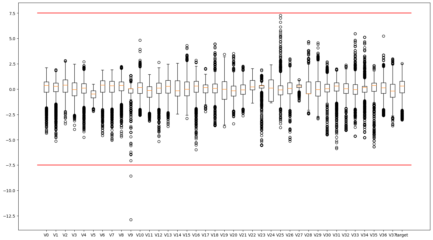
删除异常值
1 | |
归一化
1 | |
查看数据分布情况
查看特征’V5’, ‘V17’, ‘V28’, ‘V22’, ‘V11’, ‘V9’数据的数据分布
1 | |
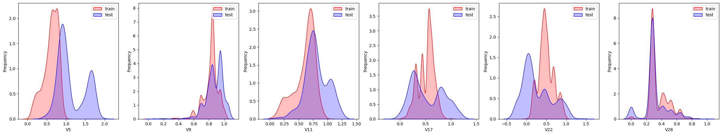
这几个特征下,训练集的数据和测试集的数据分布不一致,会影响模型的泛化能力,故删除这些特征
特征相关性
1 | |

特征降维
相关新分析
1 | |
target    1.000000
V0        0.712403
V31       0.711636
V1        0.682909
V8        0.679469
V27       0.657398
V2        0.585850
V16       0.545793
V3        0.501622
V4        0.478683
V12       0.460300
V10       0.448682
V36       0.425991
V37       0.376443
V24       0.305526
V5        0.286076
V6        0.280195
V20       0.278381
V11       0.234551
V15       0.221290
V29       0.190109
V7        0.185321
V19       0.180111
V18       0.149741
V13       0.149199
V17       0.126262
V22       0.112743
V30       0.101378
Name: target, dtype: float64
相关性初筛
1 | |
   features_and_target      corr
0               target  1.000000
1                   V0  0.712403
2                  V31  0.711636
3                   V1  0.682909
4                   V8  0.679469
5                  V27  0.657398
6                   V2  0.585850
7                  V16  0.545793
8                   V3  0.501622
9                   V4  0.478683
10                 V12  0.460300
11                 V10  0.448682
12                 V36  0.425991
13                 V37  0.376443
14                 V24  0.305526
多重共线性分析
1 | |
[216.73387180903222,
 114.38118723828812,
 27.863778129686356,
 201.96436579080174,
 78.93722825798903,
 151.06983667656212,
 14.519604941508451,
 82.69750284665385,
 28.479378440614585,
 27.759176471505945,
 526.6483470743831,
 23.50166642638334,
 19.920315849901424,
 24.640481765008683,
 11.816055964845381,
 4.958208708452915,
 37.09877416736591,
 298.26442986612767,
 47.854002539887034]
PCA降维
1 | |
| 0 | 1 | 2 | 3 | 4 | 5 | 6 | 7 | 8 | 9 | 10 | 11 | 12 | 13 | 14 | 15 | target | |
|---|---|---|---|---|---|---|---|---|---|---|---|---|---|---|---|---|---|
| count | 2.886000e+03 | 2.886000e+03 | 2.886000e+03 | 2.886000e+03 | 2.886000e+03 | 2.886000e+03 | 2.886000e+03 | 2.886000e+03 | 2.886000e+03 | 2.886000e+03 | 2.886000e+03 | 2.886000e+03 | 2.886000e+03 | 2.886000e+03 | 2.886000e+03 | 2.886000e+03 | 2884.000000 |
| mean | -8.309602e-17 | -5.653059e-17 | 7.698662e-17 | 1.023282e-16 | 1.123303e-17 | -2.096575e-17 | 1.186440e-16 | 2.303347e-17 | -8.889286e-17 | 7.044204e-17 | 2.085635e-17 | 7.888604e-17 | 1.061271e-17 | -8.522866e-17 | -3.927472e-18 | 1.403527e-16 | 0.127274 |
| std | 3.998976e-01 | 3.500240e-01 | 2.938631e-01 | 2.728023e-01 | 2.077128e-01 | 1.951842e-01 | 1.877104e-01 | 1.607670e-01 | 1.512707e-01 | 1.443772e-01 | 1.368790e-01 | 1.286192e-01 | 1.193301e-01 | 1.149758e-01 | 1.133507e-01 | 1.019258e-01 | 0.983462 |
| min | -1.071795e+00 | -9.429479e-01 | -9.948314e-01 | -7.103085e-01 | -7.703982e-01 | -5.340293e-01 | -5.993765e-01 | -5.870824e-01 | -6.282791e-01 | -4.902512e-01 | -6.340717e-01 | -5.906511e-01 | -4.174969e-01 | -4.310403e-01 | -4.170661e-01 | -3.599371e-01 | -3.044000 |
| 25% | -2.804085e-01 | -2.613727e-01 | -2.090798e-01 | -1.945196e-01 | -1.315622e-01 | -1.264097e-01 | -1.236367e-01 | -1.016457e-01 | -9.662180e-02 | -9.297320e-02 | -8.202288e-02 | -7.721862e-02 | -7.139615e-02 | -7.473615e-02 | -7.710889e-02 | -6.599455e-02 | -0.348500 |
| 50% | -1.417104e-02 | -1.277241e-02 | 2.112159e-02 | -2.337402e-02 | -5.122768e-03 | -1.355318e-02 | -1.749546e-04 | -4.655494e-03 | 2.574985e-03 | -1.480464e-03 | 7.296441e-03 | -5.733519e-03 | -4.165757e-03 | 1.036940e-03 | -1.762762e-03 | -7.954922e-04 | 0.313000 |
| 75% | 2.287306e-01 | 2.317720e-01 | 2.069571e-01 | 1.657590e-01 | 1.281659e-01 | 9.993165e-02 | 1.272086e-01 | 9.657155e-02 | 1.002626e-01 | 9.059782e-02 | 8.835004e-02 | 7.147987e-02 | 6.785346e-02 | 7.576130e-02 | 7.115629e-02 | 6.364658e-02 | 0.794250 |
| max | 1.597730e+00 | 1.382802e+00 | 1.010250e+00 | 1.448007e+00 | 1.034062e+00 | 1.358963e+00 | 6.191591e-01 | 7.370069e-01 | 6.449190e-01 | 5.839583e-01 | 6.404954e-01 | 6.780797e-01 | 5.156587e-01 | 4.977880e-01 | 4.675102e-01 | 4.571981e-01 | 2.538000 |
模型训练
1 导入相关库
1 | |
2 切分数据
对训练集进行切分,得到80%的训练数据和20%的验证数据。用切分得到的训练数据训练模型,用切分得到的验证数据评估模型的性能优劣。
1 | |
3 多元线性回归模型
1 | |
LinearRegression: 0.271697499977603
优点:模型简单,部署方便,回归权重可以用于结果分析;训练快。
缺点:精度低,特征存在一定的共线性问题。
使用技巧:需要进行归一化处理,建议进行一定的特征选择,尽量避免高度相关的特征同时存在。
本题结果:效果一般,适合分析使用。
4 K近邻回归
1 | |
KNeighborsRegressor: 0.2734753438581315
优点:模型简单,易于理解,对于数据量小的情况方便快捷,可视化方便。
缺点:计算量大,不适合数据量大的情况:需要调参数。
使用技巧:特征需要归一化,重要的特征可以适当加一定比例的权重。
本题结果:效果一般。
5 随机森林回归
1 | |
RandomForestRegressor: 0.2477930646584775
优点:使用方便,特征无须做过多变换;精度较高:模型并行训练快。
缺点:结果不容易解释。
使用技巧:参数调节,提高精度。
本题结果:比较适合。
6 LGB模型回归
1 | |
[LightGBM] [Warning] Auto-choosing col-wise multi-threading, the overhead of testing was 0.000303 seconds.
You can set `force_col_wise=true` to remove the overhead.
[LightGBM] [Info] Total Bins 4080
[LightGBM] [Info] Number of data points in the train set: 2308, number of used features: 16
[LightGBM] [Info] Start training from score 0.119128
lightGbm:    0.2436390703800861
优点:精度高。
缺点:训练时间长,模型复杂。
使用技巧:有效的验证集防止过拟合;参数搜索。
本题结果:适用。
工业蒸汽预测-04模型训练
https://blog.966677.xyz/2023/08/01/工业蒸汽预测-04模型训练/